
Apply Conditional Formatting to Pivot Table
Apply Formatting to Pivot Table Cells
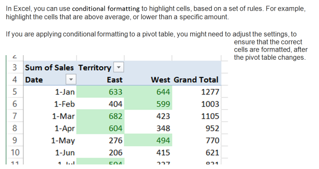
In a pivot table with a simple layout, you can select a group of cells, and apply a conditional formatting rule. In this example, the Date field is in the Rows area, Territory is in the Columns area and Sales Amount is in the Values area.
We want to highlight the sales amounts that are above average. The Grand Total amounts won't be included, because they would skew the average.

To apply conditional formatting:

The cells with above average values are highlighted.

Problems After Updating the Pivot Table
When you apply conditional formatting to a block of cells in the pivot table, the formatting rule is applied to those cells only.
If you change the pivot table layout, or add new records to the source data, the rule may be applied to the wrong cells, or might not include all the new data.
Follow these steps to add new data, and see what happens to the formatted cells in the pivot table.

The new data appears in the pivot table, but it does not have the conditional formatting rule applied, because it is outside of the original block of cells.

Change the Formatting Range
To ensure that the correct range is formatted, you can change one of the settings.


No comments:
Post a Comment