Excel Drop Down lists

There are three different types of drop-down list available in Excel, "Pick from" lists which are generated automatically, Data Validation lists which are very easy to do and, finally, Combo box and List box controls which require a bit more work. 

Pick from lists

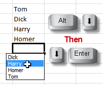
As you type a list of data into a column in your worksheet you are automatically prompted with previously entered list elements that match your typed characters. In the illustration, I have typed in an "f" and the cell is filled-in with "fred" as this entry is already in the list.

To accept the prompted text, press ENTER or press the Down Arrow key. To decline the suggestion, keep typing.

ALT Down Arrow displays the list

To generate the list entries without your having to do any initial typing, you can use the shortcut key combination ALT + Down Arrow to display the list elements and then, if you're a keyboard fan, press the Down Arrow key again to go down through the list and then ENTER to accept the entry.

If you can't be bothered with all this good old-fashioned shortcut keys business then just right-click in the cell and choose Pick from Drop-down list in the shortcut menu.

Right-click menu

Data Validation lists

These lists are used where you want to restrict the entry made in a cell to only those items available in a drop-down list. The list of valid entries can be typed in or you can refer to a range of cells which contains your valid entries.  The range of valid entries can be entered into a different worksheet in the same workbook.

Data Validation

Data Validation lists are ideal not only where you need to make sure that people make the right entry but also for data entry generally as it is so easy to choose from a drop-down list. To create the validation list, select the cell or range of cells where you want the list to be displayed and then click the Data Validation control on the Data tab (look for Data Validation in the Data menu if you are using an older version of Excel)

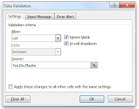In the Settings tab, choose List from the Allow drop-down list and then type in a comma-separated list of your valid entries into the Source box. Click the OK button and you're done. The list is available when you click on one of the cells where the validation has been applied and data entry in the cell is restricted to only those items in the list. Click the Error Alert tab if you want to change the standard "the value you entered is not valid" error message for invalid entries. You may prefer something a little more personal. 

Using a range of cells to provide the source

Range of cells

A range of cells is preferable for your data validation where you either have a long list or you want to be able to change the list regularly.

You can set the Source data validation as either a horizontal or vertical range of cells or an entire column or row. Either type in the range reference or (far easier) select the range or click the column letter or row number.

If you click the column letter then remember that any heading at the top of your list on the worksheet will be included as the first item in your validation list. But if you add to the list on the worksheet then these additional items will automatically appear in the validation list. So there are advantages and disadvantages to selecting the whole column.

If you specify a range of cells then then you don't have the headings issue to deal with but if you then add to the list on the worksheet then you will also have to remember to reset the Source data range to include your additions.

Referring to a range on a different worksheet

If you are using Excel 2010 or later then when you set the validation source range as being a range which is entered on a different worksheet, simply click the relevant sheet tab and then select the range. No Problem. Should you have an earlier version of Excel then you have a problem as you won't be able to click any other sheet tabs and even if you type in the range reference with it's sheet reference it will not be accepted! Don't despair, it can be done but it's a wee bit clunky.

Referring to a range on a different worksheet for older versions of Excel

If you have any version of Excel before Excel 2010 then you have to firstly Name the range of cells that you want to use for your validation source data range and then refer to that Named Range when you do the data validation.

The Name Box

Firstly, select the cells containing your list and give it a suitable name using any naming method that you're familiar with. If you're not sure how to name a range then I would recommend using the Name Box, which is that area on the extreme left-hand side of the formula bar where you normally see your active cell reference.

Name the Range

Type in the name (in this example it is "Months") and then press the ENTER key to register the name correctly. Please don't click out of the box after typing the name, press ENTER! Sorry for being boring but that's where it's so easy to go wrong.

Finally, select the cells where you want to apply your data validation and then refer to the named range in the Source box. It's no good just typing in the range name, you have to make a reference to the range name. In our example, we are using the range "Months" so the reference needs to be entered like this, =Months.

Wrong!

If you leave out the equals sign in front of the name then your data validation list will display as the literal text of the name rather than the range itself.

Displaying the drop-down list in alphabetical order

The drop-down list is linked to the values in the worksheet cells, so sort the list in the cells in alphabetical order if you wish to show the drop-down list in the same order. But you can't have the drop-down list in a different order.

Dependant Data Validation lists

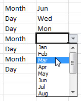
Sometimes you need the choice that you have made in one list to control the list shown in another cell; one of your validation lists is dependant on the other.

Dependant lists

In the illustration there are two columns, the first column shows the class of date required, "Month" or "Day". This is entered from a simple comma separated validation list which is typed in. The second column needs to show either a list of months if "Month" is entered in the corresponding cell in the first column or a list of days if "Day" is entered.

There are two ranges of cells in the worksheet named as Month and Day respectively which are going to be the alternative source ranges for the second column. When you set the source data range for the second column enter the following formula: =INDIRECT(A2)

Where A2 is the first cell in the first column where you have your "Day" or "Month" entry. Of course, you should change this cell reference to suit your own worksheet. The INDIRECT function is well named as it makes the reference indirect, i.e. not A2 but the range reference entered in A2. In other words, if it's "Day" then show the Day list, if it's "Month" then show the Month list. You're not restricted to just having a choice between two alternative lists, with this method you can have the choice of as many different lists as you like.

If this does not seem to work for you then try checking the following points:

1. Did you select the area for the dependant range before applying the Data Validation? In the example above it would have been the second column. It's very easy to apply validation to a single cell when you intended to set it for a range.
2. Check the spelling of the range names (in this case "Day" and "Month") in the first list. They must be correct and you have to remember them as you type them in.

Combo box and List box controls

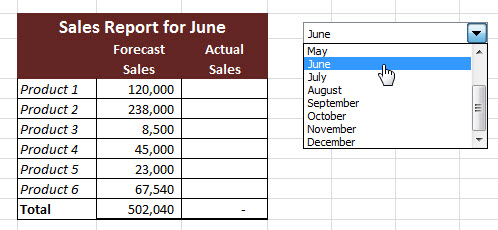
These are interactive graphics which are drawn on top of the worksheet cells and then linked to certain key worksheet cells. They are commonly employed as a user-friendly graphical device to make user-unfriendly processes involving formulas much easier to control. 

Using a Form control to update worksheet data

In the above example, there is a combo box control containing a list of months. When a month is selected from the list the heading in the worksheet report is updated ("Sales Report for ...") and the relevant monthly numbers are extracted from another worksheet where the full twelve month's figures are stored.

All this is done using Excel formulas but you don't need to know anything about the formulas to use the worksheet, you just choose a month from the list. Combo box controls are quite easy to do, the hard bit is doing all the formulas.

Form controls

There are two sets of graphical controls available in Excel, Form controls and ActiveX controls. They both do much the same job but in rather different ways so it doesn't matter which set you use.

Form controls were designed and built for Excel whereas ActiveX are more general controls which are used in many different applications. Form controls are simple and robust whereas ActiveX controls are more sophisticated and the process of using them takes far longer. It's a judgement call. I shall be using Form controls in this example and deal with ActiveX in a future article.

Finding the Form controls

This is the first job. Form controls are not openly available, you need to reveal them and each version of Excel is different.

• Excel 2003 and before. Right-click any visible toolbar and choose Form controls from the shortcut menu. Form controls are on the toolbar.
• Excel 2007. You need to display the Developer tab on the ribbon. Click the Office button and then choose Excel Options. Check Show Developer tab in the ribbon in the Popular section. Form controls are in the Insert control on the Controls group of the Developer tab.
• Excel 2010 and after. You need to display the Developer tab on the ribbon. Click the File tab and then click Options. Click Customize Ribbon and then click the Developer check box in the Main Tabs list on the right-hand side. Form controls are in the Insert control on the Controls group of the Developer tab. 

Click the Insert control, the Form Controls are the top group. The Combo Box (1) control is the second one in from the left. The List box (2) control is second in from the right. Both controls behave the same; the Combo box is a drop-down list, the List box is an open list.

Creating the Combo Box

You need to go through a few steps to get the Combo box working. Firstly, create some cell ranges where you are going to store the data that you want to have displayed in the drop-down list and a cell to link the Combo box to. When you format your Combo box these ranges are going to be your Input range and your Cell link.

Personally, I would always put these data ranges on a separate worksheet so that I can then hide it. In the example I shall be using Named Ranges, as they are so easy to work with, rather than normal cell references but this is just personal preference. Use Named Ranges or the standard A1-style cell references as you prefer, they both work fine.

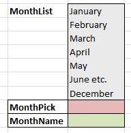Cell data ranges

In the illustration, I have a list of my twelve months (shortened for clarity) these are the grey cells and are named MonthList. The red cell is going to be the cell link and is named MonthPick and the green cell is MonthName, where I am going to enter a formula which will calculate the current month. Now it's time to create the Combo box, there's three steps:

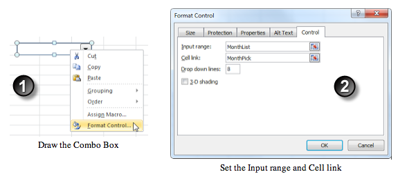
1. Draw the Combo box. Click the Combo box control and then drag to draw a horizontal rectangular shape. You can resize it later if it's not quite right. Right-click the control to display its shortcut menu. Try to right-click when your mouse pointer is pointing to the middle of the control as there are different shortcut menus available, you want the one that contains Format Control.
2. Format the Combo box. In the Format Control dialog enter the Input Range (in this example MonthList) and the Cell link (MonthPick) Click OK.
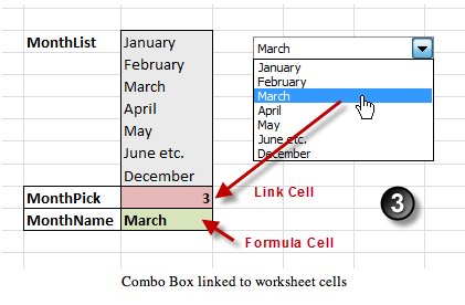
3. Test the Combo box. Click a worksheet cell to take the focus away from the Combo box. It's now active. Click the drop-down arrow and choose an item from the list. You should see that a value is returned into your link cell. It's an index value, it's not the text from the list. If you choose "March" from the list then the index is the value of 3 because it's the third item in the list.

That's the Combo box control completed and now it's time to enter our formulas in the worksheet to make everything happen.

Entering the formulas

When you choose a month from the list you want to trigger the following processes in your formulas:

1. Update the month name definition. This formula goes in the cell named MonthName so that we can use the name in our formulas wherever we need the selected month declared.
2. Update the report heading with the name of the month.
3. Update the report by showing the relevant data for the selected month.

Formula in the MonthName cell

Use the index value MonthPick to return the relevant item from the MonthList list using Excel's INDEX function. The formula is:

=INDEX(MonthList,MonthPick)

Update the report heading with the name of the month

The named range MonthName updates to show the currently selected month so we concatenate it's value with the static text "Sales Report for ...". The formula is:

="Sales Report for "&MonthName

Update the Sales Forecast figures to show the currently selected month

There's various ways of doing this but the most obvious way is to use the index value MonthPick in a Lookup formula to return the current month's figures from the range containing all the year's Sales Forecast figures.

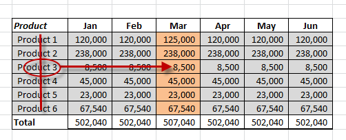Looking up the monthly figures with VLOOKUP

In the illustration, the grey cells are named SalesForecast. If the selected month was "March" then the value of MonthPick would be 3. The corresponding "March" figures are in the 4th column of the table so if we add the value of 1 to MonthPick then we can calculate the correct column index for our lookup formula. The formula is:

=VLOOKUP(B5, SalesForecast, MonthPick+1, FALSE)

Where B5 is the cell reference of the first Product in the main report, SalesForecast is the lookup range, MonthPick+1 the column index value and FALSE because it is an Exact Match VLOOKUP based on matching the product name in the main report to the products listed in the first column of the lookup range.

You might find it a bit clearer if you examine a working copy of the Excel workbook:

Download Excel workbook

Related Posts
Excel-Calculations without formulas
Excel-Sorting by last name
Excel-Switching columns to rows
Excel-Calculating age from date of birth

Training Courses

If you've still got that "I just don't know what I'm doing" feeling then you might like to arrange an Excel training course for yourself or with some of your colleagues. It's really easy to book one of our courses and they're great value for money. See our website for full details.