Excel, the CTRL key tricks

The CTRL key. That dull, grey-beige looking key that lives an unassuming, lonely life on the edge of your keyboard actually leads an exciting double life in Excel. Now, this is not going to be a life changing experience for you but it may bring a touch of fun into otherwise unexciting everyday tasks.

Copying and Moving

Copying and Moving Worksheet Cells

Drag and Drop

Cut and Paste is most peoples's favourite method of moving data from one cell to another. A simpler alternative is Drag and Drop; point to any of the cell's borders, wait for the arrow pointer to display and then drag your data to another cell.

If you want to drag your selection onto another worksheet, drag down to the sheet tabs and then hold down the ALT key to switch over to the other worksheet.

Copying cell data

To change your move into a copy (Copy and Paste), hold down the CTRL key as you drag. You should see that a plus sign is displayed next to the arrow pointer. Keep your CTRL key held down until you have released the mouse button.

Cell drag and drop is usually enabled. Should you find that the arrow pointer does not display then you need to turn it on. The settings is in Excel Options (File tab), Advanced section, Editing options: Enable fill handle and cell drag-and-drop.

Copying and Moving Columns and Rows

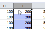
Moving a column

Drag and Drop works in exactly the same way for moving or copying entire columns or rows. Just click the column letter or row number first to select it and then point to the edge of the selection. Drag to move or CTRL+Drag to copy.

Copying and Moving Worksheets

Copying Sheets

You've already figured it out; the drag and drop method is equally effective for copying and moving entire worksheets. Point to the sheet tab and click, the document icon will display. Now drag to the left or right hand side to move the worksheet into a new position in the workbook.

To make a copy of an entire worksheet, point to the sheet tab and click. When the document icon displays, hold down the CTRL key and you will see a plus sign displayed on the icon. Now, drag the sheet to the left or right hand side to create a copy. Try doing that with Copy and Paste.

A copied sheet

On some keyboards you need to hold down the CTRL first before clicking the sheet tab.

If your worksheets are in different workbooks then you can still drag and drop your worksheets but you need to have both of the workbooks visible first. Arrange the documents on the screen by clicking the View tab,  then go to the Window group and click Arrange All, Tiled.  Drag to move a worksheet, CTRL+Drag to copy.

Copying worksheets from one workbook to another

And the Shift Key

Hold down SHIFT as you drag...

When you drag and drop one cell onto another you usually overwrite the data in the destination cell or range of cells.

But when you hold down the SHIFT key as you drag then you insert cells into the destination range without overwriting data.

...to shift cells down

Watch the I-beam as you drag, the vertical I-beam means Shift cells right and the horizontal I-beam means Shift cells down.

In the illustrations we took the 450 cell value over to the right and dragged it into the E5 cell position and the rest of the cell range moved down to accommodate the data insertion.

Filling Data with the Fill handle

Numbers

Number sequence

The Fill handle is that little black cross-shaped mouse pointer that appears at the lower right corner of the active cell. Not unreasonably, it is popularly known as the "little black cross". When you drag the Fill handle down or across you fill the data from the active cell across or down: formulas are copied, numbers are copied as constants and text stored in an Custom list, such as days of the week, triggers the list sequence.

When you hold down the CTRL key as you drag you will see a plus sign displayed on the black cross and this reverses the normal behaviour of the fill. For example, if you drag a cell containing the value of 1 then the number 1 will remain constant but if you hold down the CTRL key then you will generate the sequence of values: 1,2,3,4 etc.

Text

Custom Lists

Normal text is copied as a constant but Custom list text is entered in the order of the custom list. Custom lists can be very handy; for example you type "March" into a cell then you drag to enter the other months of the year.

But this can be irritating if you wish the month name to remain constant. This is where you hold down the CTRL key to reverse the usual action. Type in "March" and then CTRL+Drag to enter "March" into the cells below.

Excel Custom lists can be viewed, edited and set up in Options (File tab), Advanced section, scroll down to General and click the Edit Custom Lists control.

Repeating Patterns

Repeating

Sequences of numbers may be generated by creating a seed pattern in a few cells and then selecting this seed pattern and dragging to extend the sequence. For example a plus 10 sequence is seeded by typing 10 and 20 into consecutive cells, then you select the two cells and drag to generate the sequence 10,20,30,40,50 etc.

Repetitions of the seed pattern are obtained by holding down the CTRL key as you drag. The sequence of values is then repeated; 10,20,10,20,10,20 etc.

Text values can be treated in much the same way, enter and select an initial pattern of text and then CTRL+Drag to create repetitions of the original. In the illustration below, we wanted the headings "Budget" and "Estimate" repeated across the top of a financial report. Instead of Copy and repeated Pastings the headings were dragged across to the right with the CTRL key held down.

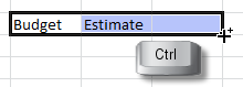
Repeating Headings

Making Selections

Cells

CTRL key for multiple selection

A multiple selection of cells is where you select one range of cells and then you hold down the CTRL key and keep it held down as you continue to add to your initial selection and create a collection.

If you make a mistake then there's nothing to be done other than to click a cell to clear your current selection and start over again.

This sort of selection is so useful for cell formatting as you can apply your formats to the entire selection in one fell swoop instead of having to format each range individually and invaluable where you want to plot cell ranges which are not immediately adjacent to each other on an Excel chart.

Columns and Rows

Adjusting the width of alternate columns

The same method of selection is easily applied to entire columns or rows by clicking the first column letter or row number, then you hold down the CTRL key and click on the others.

With multiple rows selected you can apply actions such as deletion to all the selected rows or with multiple columns selected, as in the illustration, you can change the width of alternate columns in your worksheet. The more you use collections the more ideas you will have. Not all actions can be applied to a multiple selection but it is always worth experimenting.

Worksheets

In the illustration below we coloured alternate sheet tabs red in one go by holding down the CTRL key and clicking on the relevant sheet tabs. Right-click any selected tab to access the Tab Color command.

Colouring alternate sheet tabs

And the Shift Key again

SHIFT key for block selection

The other method of selection that is useful to know is Block selection which uses the SHIFT key. This is the selection of a continuous range of cells effected not by dragging, as is usual, but by clicking. You click the first cell of your selection, hold down the SHIFT key and then click the last cell. It's Click, Shift, Click.

This feels very awkward if you never tried it before as you can not stop yourself from dragging but if you practice the technique on small ranges of cells then you will rapidly master it. And then you can apply in so many different situations: selecting huge ranges of cells, ranges of sheet tabs etc.

Click, SHIFT, Click

Now you're an expert in the dark art of Excel cell selection you will find that you can use these selection techniques on other Excel objects and in other Microsoft Office applications. 

Extend Mode

A final word on multiple selection, using your keyboard. The CTRL key with a normal mouse is the easiest thing in the world, you hold the key down with your left hand and select with your right hand. But left-handers don't always have such an easy time of it and some touch pads can make you wish that you had a third hand. This is where you need Extend Mode with the keyboard.

Press function key F8 to open extend mode and then select your first cell range either using your mouse or by using your keyboard: hold down the SHIFT key and extend the selection by pressing your arrow keys.

Extend Selection

Now, lock your current selection by pressing SHIFT+F8 and then move on to make your next selection. This is best done by pressing the arrow keys to exit the current selection and then pressing SHIFT and arrow keys again to make the next selection. Press SHIFT+F8 again to lock this selection and continue in this way until the selection is complete.

I can assure you that this is a lot easier to do than it is to read about it.

Related Posts

Excel-The Double-click tricks

Excel-Calculations without formulas

Excel-Sorting by last name

Excel-Switching columns to rows

Excel-Calculating age from date of birth

Excel-Drop-down lists

Excel-Top Ten shortcut keys

Copying Photos to your iPad

A Fanboy's Lament

The sensible side of me resisted the iPad for so long. "What would I do with it?" I asked, sensibly. But once you've held one in your hot, little hands it's love at first sight. Resistance is futile. Like all love affairs, there is a dark side; the iPad only has a Lightning connector and I wanted to copy hundreds of photos from my camera.

The Apple Store will sell you a Lightning to SD Card Camera Reader but at a stonking 25 quid a pop it causes a sharp intake of breath. I don't know why I should be so mean when I'm looking at prices on the web while I am the world's worse retail victim when I'm browsing in the actual, physical Apple Store. I look at all their gadgets and gizmos and am happy, almost ecstatic, to find one I don't have and then eager to hand over wads of cash in return for a small, white plastic thing that may prove vaguely useful to me. Is this what they mean by being a "fanboy"?

The cheapo Lightning adapter

Or you can get one of these cheap plastic memory card readers on flea bay for a few quid. Very cheap plastic and nothing like as nice as proper, white Apple plastic.

And there's a trick to getting these adapters to work properly, you can't just shove them into your iPad and expect to copy your photos. You have to create a DCIM album on your iPad before you connect the adapter. DCIM (Digital Camera IMages if you must know) is a magic, reserved name in digital camera land as you've probably already noticed.

Making a DCIM album

So, fire up your iPad, go to your Photos app and choose Albums.  Tap the plus sign on the top left to create a New Album. Enter DCIM ("Dcim" works as well and I couldn't be bothered to test "dcim") then press Save. Slide your SD card into the card reader and plug the whole assembly into the Lightning connector. Wait 10 seconds or so and you will start to see thumbnails of all the photos stored on your SD card appear on your iPad screen.

Reading the SD card

Hum a happy tune while all the files are read and then press Import All. Your photos are imported into your Photostream, not your DCIM album. After that you can make your own albums and add photos from your Photostream. Leave your DCIM album empty.

I was using puny 2GB and 4GB SD cards and had no problems with reading the card. I would put serious money on these adapters not working with high capacity cards.

But I don't care; I'm not spending my pocket money on fancy-pancy, super-duper, high capacity SD cards. I'm saving up to buy a proper Apple card reader. A white one. Please don't tell anyone.

Related Posts

iPad- Force quit Safari when web page stuck in a loop

iPhone- Last Number Redial

Apple Mac OSX Rename files keyboard shortcut

Excel for Mac Deleting a range and other shortcut keys

Word for Mac Make your own menu

Apple Mac OSX Recovery startup keys

Excel, the Double-Click Tricks

Here's a selection of my favourite double-click shortcuts for Excel. I bet you know them already. If you don't then prepare to throw your toys on the floor.

Copying a Formula Down the Column

Double-click the Fill Handle

This the best one. I wasted long years of my life dragging formulas down the column until I discovered that all you had to do was double-click the corner of the formula cell.

I did'nt know whether to laugh or cry. It's so easy. Hover your mouse over the lower right-hand corner of the cell and wait for the Fill Handle (black cross) to appear. Then double-click to copy the formula down the column.

Copy down the column

So long as there are no blank cells in the previous column your formula copies all the way down to the end. The end of what? The end of the previous column, that's why it's a really bad idea to leave a blank column between your last data column and the column used for the formulas.

This double-click to copy down method is so much better than dragging that it's usually easier to delete your blank column, do the copying and then insert the blank column afterwards.

Adjusting Column Widths

AutoFit Column Widths

This method also works with row heights but it's dealing with column width problems where it really comes into it's own.

We are all familiar with the column width problem where you have the hash signs displayed in your cells. The last thing you want to do is start dragging the column wider, instead hover your mouse over the right-hand edge of the column until the double-headed arrow appears and then double-click to apply an automatic column width. This is based on the longest entry in the column.

Remember, work on the columns and not the cells containing the hash signs. If you have several columns to adjust, which is often the case, then select them first. Click on the first column letter and then drag across to select the others. Double-click between any two columns in your selection and all the columns are done in one go.

Using the Format Painter

The Magic Paintbrush

Most of the MS Office applications have a Format Painter control which you can use to copy all the formatting from one place to another. That's ALL the formatting in one go. But just once.

What is not so obvious is that when you double-click the Format Painter you can repeat your formatting by continuing to click on additional items. The Format Painter stays on until you deliberately cancel it by pressing the ESC key or single-clicking the control.

To use the Format Painter in Excel, apply formatting to a single cell or a range of cells and then either click (to paste the formatting once) or double-click. Now, select another cell or range and all the formats (fill colours, borders, fonts, number formats etc.) are copied from the source to where you have just clicked. As you do this you will see a paintbrush image attached to your mouse pointer.

Format Painter in action

The Format Painter control is found on the Clipboard group (on the extreme left-hand side) of the Home tab. In older versions of Excel the Format Painter tool is on the Standard Toolbar.

I laugh at myself every time I use the Format Painter as I used to think that the brush image meant "Paste" and I could not seem to get Copy and Paste to work properly. Then I learned Ctrl+C and Ctrl+V but I still used to copy my formats using the menu; Edit, Paste Special, Formats. Really sad.

Movement and Selection

You can double-click the border of the active cell to move it in any direction to the end of the current block of cell data.

Double-click the lower border and you move down, left border and you move left, right border to move right etc. You always stop at the first blank cell.

Instead of moving the current active cell, to select the range of cells down or across, hold down the SHIFT key as you double-click one of the borders. You expand your current selection down or across to the first blank cell.

Using the Keyboard

You can do all of this with the keyboard if you prefer. To move the active cell, press the END key and take your finger off it. Excel is now in END mode. Now, press any one of the four arrow keys to move in that particular direction.

Practice using the END key sequence a few times and then you can bring your SHIFT key into play to make selections. Hold down the SHIFT key and keep it held down as you press any one of the END and arrow key sequences.

Related Posts

Excel-the CTRL key tricks

Excel-Calculations without formulas

Excel-Sorting by last name

Excel-Switching columns to rows

Excel-Calculating age from date of birth

Excel-Drop-down lists

Excel-Top Ten shortcut keys

Excel Converting USA Dates to UK Dates

Converting USA Dates to UK Dates

Usually Excel date values don't cause any problems, you type them in with slash or dash separators and don't bother about the year value unless your date is for a year other than the current year. Excel automatically enters the current calendar year if you just give day and month values. 

Excel Date Converter

But you will have a problem if the country setting on your system has not been set correctly. Excel was written in the USA and uses their Month-Day-Year date convention so you will have to change it if you want to use the UK convention of Day-Month-Year.

The United States Declaration of Independence is clearly dated "July 4 1776" and there's little chance of their changing to suit us. You can't argue with the Founding Fathers.

The country setting issue is easily resolved, the real date problem arises when you have to share documents with your friends and colleagues from across the pond. Your opposite number in New York emails you data that was quite sensible when it was entered but when you open the document the dates go haywire. 

Happy dates!

You can Google formulas that will reverse the date evaluation for you but they are awkward to implement if you have to do this sort of thing regularly. In this article we are going to create a Date Converter that reverses the day and month values of any date directly in the cell without having to use formulas. The converter uses an Excel macro which is triggered when you click a shortcut button on your Quick Access Toolbar (QAT).

Converting UK Dates to USA Dates

It also works the other way round. So, if someone from the London office sends you a spreadsheet and the dates are entered in good-old-King-George Day-Month order you select your cells, click your shortcut and it whizzes the date evaluation around into nice, sensible Month-Day dates. 

Making the Date Converter macro

There's ten steps to go through here but don't let that put you off as they are very simple and the entire process will only take a few minutes. If you're not familiar with the term "macro" then allow me to explain. Macro is short for macro-instruction and is a sequence of instructions written in Excel's scripting language, VBA (Visual Basic for Applications)

Step 1. Recording a macro

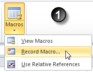
Turning on the recorder

The first step is to record a macro into your Personal Macro Workbook. This is a hidden workbook that is opened automatically whenever Excel starts up, any macros saved in this workbook will always be available for you to use.

Go to the Macros control which is found on the extreme right-hand side of the View tab on the Excel ribbon. Click the bottom section of the control and choose Record Macro from the menu.

Step 2. Using the Personal Macro Workbook

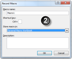
Recording a macro

There is very little to do here other than to make sure that you record a macro in the right place.

When the dialog is displayed, change the Store macro in setting to Personal Macro Workbook. It's available in the drop down list. Don't bother with anything else. Click OK to start the recorder.

Whatever you do now gets recorded but there's no need to do anything. Just turn off the recorder and this step is completed. Click Stop Recording in the menu on the Macros control.

Step 3. Finding the recorded macro

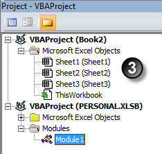
Project Explorer Window

We have now created a module (Excel's storage area for macros) in the Personal Macro Workbook. The next step is to find this module, remove the recording and replace it with the instructions that will do the date conversion work for us.

This is done in the Visual Basic Editor. Press ALT+F11 to open the editor and then see if you can spot a window in the top left-hand corner which looks like this illustration. That's the Project Explorer window. If you can't see it, press Ctrl+R.

Look in the listing under PERSONAL.XLSB, you may have to click the plus sign nodes to open up the listing. If you've never used the Personal Macro Workbook before you will need Module1. If there are a set of modules visible then you need the last one. Double-click the module and you will display the code of your recording in the window on the right-hand side of the screen.

Step 4. Copying and Pasting the code for the macro

The recorded code

Your recorded macro code will look something like this illustration. Don't worry if it doesn't as we are going to delete it and substitute our own code.

Select all your code from the word Sub to the words End Sub and press the DELETE key.

Then copy and paste the code from the section below to replace the original.




This is the code for the date macro:

Public Sub DateConverter()

    Dim rngCells  As Range

    Dim rngCell   As Range

    Dim strMsg    As String

    Dim intDay    As Integer

    Dim intMonth  As Integer

    Dim intYear   As Integer

    Dim DateValue As Date

    

    On Error Resume Next

    

    strMsg = "Select the cells to convert:" & _

                  vbCr & vbCr & "Reverses Month and Day date evaluation," _

                  & vbCr & "i.e. MM-DD becomes DD-MM if possible."

    'Receive the input.

    Set rngCells = Application.InputBox(strMsg, "Date Converter", , , , , , 8)

    

    'Test for no input received.

    If Not IsObject(rngCells) Or rngCells Is Nothing Then

       GoTo Exit_DateConverter

    End If

    

    'Date Conversion Loop.

    For Each rngCell In rngCells

        If IsDate(rngCell) Then

            intDay = Day(rngCell)

            intMonth = Month(rngCell)

            intYear = Year(rngCell)

            DateValue = intMonth & "/" & intDay & "/" & intYear

            rngCell.Value = DateValue

        End If

    Next

Exit_DateConverter:

End Sub

Make sure that you copy and paste everything, starting with the word Public and ending with words End Sub. When you've pasted the code you will see that some of the words will turn a blue colour and some green. That's exactly what they should do.

Step 5. Saving the macro

Don't forget to save!

Now save the workbook. PERSONAL.XLSB is a hidden workbook so save it now as it's tricky to do it later. Choose File, Save from the main menu.

The macro is completed and we now get back to Excel by pressing ALT+F11 again. Or you can close the Visual Basic Editor window.

Step 6. Creating a shortcut for the macro

Customize the QAT

In the next few steps we shall create an attractive, easy to use shortcut for the macro.

The most obvious place to have this is on your Quick Access Toolbar. Point to the QAT (top left-hand corner of the Excel window), right-click and choose Customize Quick Access Toolbar from the shortcut menu.

Step 7. Customizing the Quick Access Toolbar

Choose from the Macros category

Excel's Options dialog will display and the Quick Access Toolbar section is activated.

Working from the top left-hand corner of the section, click the Choose commands from drop-down list.

Then click Macros in the list.

Step 8. Assigning the macro to the QAT

Adding your macro to the QAT

Your macro will be displayed in the list on the left-hand side. Select the macro and click the Add command button.

Your macro now appears in the right-hand list which shows you all the shortcuts available on your Quick Access Toolbar.

The next step is cosmetic and will make your shortcut button more visually attractive. Click OK now if you want to skip this final step.

Step 9. Modify the macro button

Assigning an icon to your macro

Click the Modify command button if you want to change the icon displayed for your macro and change the descriptive 'Screen-Tip' that pops up whenever you point at the icon.

There's an array of different icon images to choose from. Enter some text into the Display Name box to set the Screen-Tip text.

You don't have to enter "Date Converter", you can enter anything you like. Click OK to close the dialog and OK again to close the main Options dialog.

Step 10. Test the macro

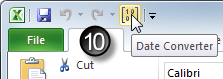
The Date Converter shortcut

Everything's done but you always want to test it to make sure. Enter a few dates into your worksheet. Click the Date Converter button on your Quick Access Toolbar. Select the date cells when the input box appears. Click OK and all the dates get switched around. Reee-sult!

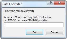
Date Converter Input Box

This is the input box that appears when the shortcut is clicked. It does not pick up your current selection- you point out of the box and select a range of cells or a column on your worksheet. All the dates in the selection have their month and day values reversed. Anything that is not a date is ignored.

Any requests

Leave a comment if you found this Step-by-Step useful and I'll post some more. I have loads of Excel  macros in my box of tricks, mainly things that I have found really handy over the years. Like, for example, password protecting all the worksheets in the workbook, protecting all the formulas in a worksheet, listing all the validation formulas used etc. Or anything else you can think of...

Happy clicking!

Microsoft Excel 2010 Shortcut Keys

If you're looking for a full listing of all the shortcut keys for Microsoft Excel 2010 you'll find them in the first issue of the Charis Alexandra Training Newsletter. Over the next few months we shall be publishing comprehensive lists of shortcut keys etc. and reproducing some of the more popular articles from this blog in a handy, printable pdf format.

Excel shortcut keys

All the back numbers of the newsletter will always be freely available on our website and you are very welcome to share the link with your friends and colleagues. Of course, you might want to sign up to receive our newsletter as it is published.

Don't worry about being spammed. Our email security policy is quite clear, we will not share your details with any third parties. Ever! That's a guarantee. You can unsubscribe whenever you like.

Watch out for the next issue, it's our Microsoft PowerPoint special. Top Tips and ALL the shortcut keys. 

Excel Top Ten shortcut keys

Top Ten Shortcut Keys

Ask ten people what their favourite Excel shortcut keys are and you'll get ten different answers. In no particular order, here's my personal choice of the ones that I can't do without. I'm not going to list ALL the Excel shortcut keys here because there are hundreds of them.

You can find a full listing of all the Microsoft Excel 2010 Shortcut Keys in our newsletter.

Ctrl+A  Select the Current Region

Select Current Region

Click a cell, press Ctrl+A and Excel expands your selection to select the Current Region. Press Ctrl+A again and the entire worksheet is selected.

The Current Region is defined as the current area of continuous data bounded by blank cells. In older versions of Excel you may have to press the key combination Ctrl+* to achieve the same effect (Ctrl+SHIFT+* if you don't have a dedicated * key)

Ctrl+Spacebar  Select the Current Column

Select Current Column

What, pick up my mouse and click the column letter. No way! Ctrl+Spacebar selects your current column and then to extend the selection to the left or right you hold down the SHIFT key and use the Left or Right arrow key.

SHIFT+Spacebar  Select the Current Row

Select Current Row

Well, I did say that it's a personal choice. Lazy-bones here selects the current row with SHIFT+Spacebar. Then keep the SHIFT key held down and press the Up or Down arrow keys to extend the selection up or down.

Ctrl+D and Ctrl+R  Fill Down and Fill Right

Fill Down

Fill formulas or data down the column by selecting down with the SHIFT and Down arrow key. Then Ctrl+D fills down the selection. Ctrl+R to fill across to the right.

Ctrl+`  Show/Hide Formulas

Show/Hide Formulas

You can't check that you've got your formulas entered correctly if you can't see them.

Switch between displaying the returned results of your formulas and the actual formula itself by pressing Ctrl+` (that's  usually the key under the ESC key in the top left hand corner of the keyboard)

ALT+=  AutoSum

AutoSum

Instead of clicking the AutoSum control every five minutes ALT+= enters a sum formula into the active cell. But it only does SUM and does not give you a choice of other functions.

See my article AutoSum Revisited for a few ideas on getting the best out of AutoSum.

Ctrl+ENTER  Range Entry

Enter into a Range

Pressing the ENTER key makes an entry into your current active cell. Ctrl+ENTER makes an entry into every single cell in your current selection. Make the selection, type in your entry and then press Ctrl+ENTER.

Constants (text or numbers) and formulas can be entered into a range in a single step. Formulas give you a relative reference for each cell, so if you get the first one right then all the others will adjust accordingly.

To enter data into a discontinuous range, make a multiple selection first. Select a cell or a range of cells then hold down the Ctrl key as you add to your selection by clicking on other cells or ranges.

ALT+ENTER  Insert New Line

Force New Line

Rather than wrapping the text in the cell whenever you want to force a new line press ALT+ENTER.

This is very handy for creating Excel source data for Tables or Pivot Tables where you maybe need to have multiple lines of descriptive text for a heading but retain the integrity of the single physical header row.

F4  Absolute Reference and Repeat

Absolute Reference

When you need Absolute References (dollar signs) in your formulas press F4. Succeeding presses of the F4 key return all the permutations of absolute and relative reference: $A$1, A$1, $A1, A1.

To make a single cell reference in your formula absolute, click somewhere on the reference then press F4. For a range reference or a series of references, drag across the references first before pressing F4.

F4 has a double life, when you are in Ready mode (i.e. not editing your formulas) F4 means Repeat. Say you have the tedious job of going through a worksheet and deleting some of the rows, delete the first one as you usually do and then select the next row to be deleted and press F4 to repeat the row deletion.

F11  Chart

Plot Chart from current selection

Pressing F11 plots a default chart on a separate chart sheet based on your current cell selection. Press ALT+F11 for an embedded chart on the active sheet.

Excel will automatically execute a current region selection if you start with a single cell selected in your chart data range.

To plot discontinuous ranges, make a multiple selection using your Ctrl key before pressing F11.





What's your favourite Excel shortcut key?

Download Excel 2010 Shortcut Keys as pdf

Related Posts

Excel-Calculations without formulas

Excel-Sorting by last name

Excel-Switching columns to rows

Excel-Calculating age from date of birth

Excel-Drop-down lists

Training Courses

If you've still got that "I just don't know what I'm doing" feeling then you might like to arrange an Excel training course for yourself or with some of your colleagues. It's really easy to book one of our courses and they're great value for money. See our website for full details.

Word Random Text

Generating random text for Word and PowerPoint

Lorem ipsum sit amet...

Do you ever need filler or placeholder text for Word documents or PowerPoint text boxes? It's quite handy when you want to plan the design and layout of your document and check out different fonts and formatting options etc.

Being an expert typist, I always used to type in double-encrypted blah, blah nonsense like this, "jkhj kefhkfh kjhjkhf hfshf jhkjhs" until I discovered random text functions. However, my typing speed has suffered, I was quite impressive typing "jkhj kefhkfh kjhjkhf" but now I'm back in the land of hunt and peck.

To generate some random text, click on your document or on a text box, type in =RAND( ) and then press the ENTER key. You get three paragraphs of random text. If you have a classical bent then you may prefer some Latin, in which case type in =LOREM( ) and you get three paragraphs of lorem ipsum. Don't forget the equals sign at the start and both the brackets at the end.

What does the filler text "lorem ipsum" mean?