One Drive for Business Help Guide

Managing your files in OneDrive for Busines

 

 

 

Credits

Microsoft Office Training Centre

Editorial

Charis Alexandra Training

 

Managing your files in OneDrive for Business

After you sync your OneDrive for Business files with your computer, you can put away your browser and manage your files like other files on your computer. Need to add a file to OneDrive for Business? Just drag it to your OneDrive for Business folder. You move, rename, and delete your files the same way you're used to, with one important difference: the changes you make to OneDrive for Business files will sync to all your other devices. So if you delete a file here, it's deleted everywhere.

Copy or move files in OneDrive for Business

 

• In File Explorer, select the files you want to copy or move.
• Right-click the files and drag them to your OneDrive - YourCompanyName folder or to another location.

• Select Copy here or Move here on the shortcut menu.

Rename a file in OneDrive for Business

1. Right-click the file you want to rename in your OneDrive - YourCompanyName folder.
2. Select Rename on the shortcut menu.
3. Type the new name for your file.

 

Delete a file in OneDrive for Business

• Select the file you want to delete in your OneDrive - YourCompanyName folder.
• Press Delete on your keyboard.

Tip   Remember, any changes you make to a file in your OneDrive for Business folder apply to all devices, not just to this computer. The changes will sync to all your other devices.

Dragging and dropping files to OneDrive for Business

You can upload files to your OneDrive for Business by just dragging them from your computer. OneDrive for Business shows you where you can drag and drop files to add files to a library.

• At the top of the page, select the Office 365 app launcher, and then select OneDrive.

• Find the documents that you want to upload on your computer and drag them to your OneDrive for Business.

Notes   

• The first time you click OneDrive, you see some setup screens and instructions while your personal site is being set up. You may have to wait awhile and then click OneDrive again before continuing to step 2.
• If you don’t see the option to drag files, update your copy of Office.
• The Edge browser doesn't support drag and drop into OneDrive for Business. Internet Explorer 11 is supported.

Here’s another way to upload files:

• Instead of dragging files, select Upload.

In OneDrive for Business you can choose Files. Use the Open dialog box to select the files you want to upload, and then click Open.

For SharePoint Online use the Add a Document dialog box. Click Browse and select the files you want to upload. Click Open and then click OK.

 

Note   You can only drag and drop, or upload files in OneDrive for Business or SharePoint Online. If you need to upload folders, consider syncing the folder with your computer. For more information on syncing, see Sync OneDrive for Business or site libraries to your computer

Tip   Your files are private unless you decide to share them. To share files easily with everyone in your organization, drag them to your Shared with everyone folder. For more information, see sharing files with others.

Seeing your files from other devices

After you upload files to OneDrive for Business, you can see them from other devices by just signing into your Office 365 site in your browser, and then clicking OneDrive. Here are the details.

• On any device, sign in to Office 365 with your work or school account. For example, ellen@contoso.onmicrosoft.com, ellen@contoso.edu, or ellen@contoso.com. If you're not sure what your work or school account is, check the welcome email that asked you to sign in the first time.

• At the top of the page, select OneDrive. Or, select the app launcher , and then select OneDrive.

• The files you upload from any device are right there for you to use.

Tip   Your files are private unless you decide to share them. To share files with everyone in your organization, upload or move them to your Shared with Everyone folder. For more about sharing, see Sharing files with others.

Set up Office Mobile on your phone or tablet

To get your Office Mobile apps to work with Office 365, choose your device.

 

Saving and opening files

You can work with the files you store in OneDrive for Business right from Word, Excel, PowerPoint, and other Office desktop apps. There's no need to go to your Office 365 site in a browser.

Save a file to OneDrive for Business from an Office desktop app

With a document open in an Office desktop app, click File > Save As > OneDrive - YourCompanyName. For example, OneDrive - Contoso.

• Browse to the location where you want to save the file, and then click Save.

Open a OneDrive for Business file from an Office desktop app

• In an Office desktop app, click File > Open > OneDrive - YourCompanyName. For example, OneDrive - Contoso.

Browse to the file you want to open, and then click Open.

Tips   If you don't see OneDrive - YourCompanyName, click Add a Place > Office 365 SharePoint. Then sign in to Office 365 with your work or school account.

Once you add OneDrive for Business as a place in one Office app, you can save files from all your Office apps.

Syncing your files with your computer

Sync OneDrive for Business to your computer, and then get to your files in File Explorer instead of in a web browser. All your changes sync to OneDrive for Business whenever you’re online.

• At the top of the page, select OneDrive. Or, select the app launcher , and then select OneDrive.

• On your OneDrive for Business page, click Sync.

• At the prompt, click Sync Now to start the sync app.
• The app automatically fills out the name and web address of your OneDrive for Business library.
• Select Sync Now in the app to start syncing.
• You can click Show my files in the app to open the synced OneDrive for Business folder in File Explorer. The folder appears in your Windows Favorites as OneDrive for Business or OneDrive - YourCompanyName.

Note   To sync files to your computer, you need the OneDrive for Business sync app, available with an Office 365 subscription that includes Office 2013 desktop applications. If you don’t have Office 2013, you can download the OneDrive for Business sync app.

Managing your files in OneDrive for Business

After you sync your OneDrive for Business files with your computer, you can put away your browser and manage your files like other files on your computer. Need to add a file to OneDrive for Business? Just drag it to your OneDrive for Business folder. You move, rename, and delete your files the same way you're used to, with one important difference: the changes you make to OneDrive for Business files will sync to all your other devices. So if you delete a file here, it's deleted everywhere.

Copy or move files in OneDrive for Business

• In File Explorer, select the files you want to copy or move.
• Right-click the files and drag them to your OneDrive - YourCompanyName folder or to another location.

• Select Copy here or Move here on the shortcut menu.

Rename a file in OneDrive for Business

• Right-click the file you want to rename in your OneDrive - YourCompanyName folder.
• Select Rename on the shortcut menu.
• Type the new name for your file.

Delete a file in OneDrive for Business

• Select the file you want to delete in your OneDrive - YourCompanyName folder.
• Press Delete on your keyboard.

Tip   Remember, any changes you make to a file in your OneDrive for Business folder apply to all devices, not just to this computer. The changes will sync to all your other devices.

Sharing files with others

• When you store your files in OneDrive for Business, you can share with others from any device by going to your Office 365 site in a browser.
• You can also share a Word document, PowerPoint presentation, or Excel spreadsheet right from within Office without even going to Office 365 in a separate window. Whichever way you choose to share Office files, you can work with others at the same time they work on a file and see the changes that other people make as they make them.

Share a file from a site

• At the top of the page, select OneDrive. Or, select the app launcher , and then select OneDrive.

• Select the file you want to share, and then select Share.

• In the Share window, type the name of each person you want to share the file with. As you type each name, suggestions appear that match your contacts. When you see the name you want, select it to add it to the invitation list.

Tip   To share files with everyone in your organization, type Everyone instead of the name of a person.

• Select the permission in the list that you want to grant people.
• You can change the permission later for any person.
• If you want, type a message to send to all the people you're inviting.
• The email message sends a link to the shared document.
• If you don't want to send an email to invitees, clear Send an email invitation.
• Click Share.

Share a file from an Office desktop app

• With the file open in Word, Excel, PowerPoint, or another Office app, click File > Share > Share with People.

• in the Share dialog, click Share with people.

• Type the name of each person you want to share the file with. As you type each name, suggestions appear that match your contacts. When you see the name you want, select it to add it to the invitation list.
• Select the permission in the list that you want to grant people.
• You can change the permission later for any person.
• If you want, type a message you want to send to all the people you're inviting.
• The email message sends a link to the shared document.
• Click Share.

Work on files with others at the same time

• When you store and share your files in OneDrive for Business, you can work with others at the same and avoid reconciling multiple versions of your files. Work together from either the online or the desktop versions of Word, PowerPoint, or OneNote. For workbooks, use Excel Online. If someone opens the workbook in the Excel desktop application, the workbook can’t be edited in Excel Online until it’s closed again in desktop Excel.

Here are a few details to keep in mind as you work with others:

• In the desktop programs, co-authoring works best in the most recent version of Office (Mac and Windows), but is also supported in Office 2010.
• There's no special co-authoring mode and no command to begin working together on a document. Just open the file for editing and start working.
• As you edit, the Office app tells you when other people are working too. In Word, you'll even see which paragraph they’re working on.
• Updates are handled differently in some programs from others. For example, OneNote notebooks and Excel Online workbooks show updates immediately. In Word documents, save the document to share your updates and to see others’ updates.

 

PowerPoint Pro Tips

Layered Objects on a crowded slide

Layered Objects

Do you ever have to deal with those crowded PowerPoint slides? You know; the ones with layers of overlapping shapes and text boxes—and you need to change the one in the middle of the pile. Some people move all the other objects out of the way so that they can see the one they want. Then they make a few changes and then move them all back again in to, hopefully, their original positions.

There has to be a better way. You can use the keyboard shortcuts Tab and Shift+Tab to cycle forward and backward through the stack of objects until you can see that the selection handles are around the one you want. Or, you can press Alt+F10 and turn on the...

Selection and Visibility Pane

There’s a control to turn this on and off on the Home tab but it’s easily missed. The Selection and Visibility Pane lists all the objects on your slide and you use it to identify and work on any object. Just click the Hide All button and then start clicking the eyes to the right to show selected objects, you’ll soon find the one you want. Make your changes, click the Show All button and you’re done. It’s so easy when you can see what you’re doing.

Selection and Visibility Pane ALT+F10

You will notice that PowerPoint uses its own fiendish naming scheme for all your objects, things like Rectangle 5, TextBox 4, AutoShape 22 make perfect sense until you have to animate them and then you have real problems trying to identify specific objects. All you have to do is rename them here according to their appearance and purpose and you’ll have a much easier time creating animations.

An object named something like Blue Box or Red Star is a lot easier to deal with than Rectangle 5. To rename an object, click the current name in the pane and replace the text.

Ruler, Gridlines and Guides

Are you still eyeballing objects on your slides to line them up? PowerPoint’s Smart Guides pop up when you are aligning objects and are a great help but for a slick and professional appearance you need to arrange your objects with precision. You need to see what you’re doing and see where things are. In short, you need gridlines, guides or your ruler, maybe all three. You’ll find them on the View tab or you can press the shortcut keys:

Rulers, Gridlines and Guides

Press Shift+F9  to show or hide the gridlines. Press Alt+F9  to show or hide guides. Press Alt+Shift+F9 to show or hide the ruler. The ruler appears around the top and left of the slide and is ideal for sizing and positioning, the grid is a design grid used to precisely align objects in relation to each other and the guides give you your centre lines.

Moving, Resizing, Rotating and Nudging Objects

You can use your mouse to move objects around but for fine control you should use the arrow keys on your keyboard. Click the object and then press any of the keys to move left, right, up or down. Hold down the Ctrl key while you press the arrow keys to nudge—move the shape in smaller increments.

Shortcuts for Resizing and Rotating

Press Shift+Right Arrow  or Shift+Left Arrow to enlarge or reduce the selected shape horizontally.

Press Shift+Up Arrow  or Shift+Down Arrow to enlarge or reduce the selected shape vertically.

Press Alt+Right Arrow to rotate the selected shape to the right.

Press Alt+ Left Arrow to rotate the selected shape to the left.

Formatting Text in Text Boxes

Are you formatting all the text in the text box or only a particular word or phrase in the text? If you are formatting all the text then there’s no need to drag across the text. Just click on the box and apply your formatting. Only select the text inside the box when you want to format just a part of it. You certainly do not want to try to select the text and end up moving the entire text box. Of course, that’s exactly what everybody does and mighty irritating is it too!

You need to be aware of your current selection. Look at the border of the text box—a solid line means the object itself is selected, a broken line means the text inside is selected. Either click the border of the box to select the object or click inside the text area to select the text. If you do this frequently then try remembering the following shortcut keys: Esc to select the text box when you have the text selected inside it. Enter to select the text inside the text box when you have the text box selected.

Text in the text box selected and the text box itself selected

Colour Matching with the Eyedropper

Colour matching

One of the best ways to create an impressive presentation is to use consistent colours. Ensuring that the various elements on your slide are the same colour creates a visual unity for your content. But it’s so hard to match colours precisely; the text on your slide needs to exactly match that shade of blue in your company logo. How do you do it?

As a design tool PowerPoint has definitely needed this for years but it was only introduced with PowerPoint 2013 so you will be disappointed with this one if you have an earlier version. PowerPoint 2013 features the Eyedropper which makes colour matching a breeze. You can match colours not only in your presentation but to any other colours on your screen.

The Eyedropper control

The Eyedropper is included on any drop-down menu that you use to pick a colour. On your PowerPoint slide, select a shape that you want to colour match and then click the Eyedropper. Move your mouse over any other object and observe the colour in the preview window beside the Eyedropper cursor. Just click when you see the desired colour to apply it to the shape.

Eyedropper cursor and RGB values

As you move your pointer around the screen a live preview of the colour appears. Hover or pause on a colour to see its RGB (Red Green Blue) colour coordinates. Click on the colour you want. To cancel without picking a colour, press Esc.

Matching the colours of PowerPoint objects on your slide to something outside of PowerPoint is just as easy. Once again, select the object that you want to colour match and, holding down your mouse’s primary button, drag to move the Eyedropper cursor outside of the PowerPoint window. You can now match any colour that you see on your screen, release the mouse to apply the desired colour.

Related Posts

PowerPoint-Balance Diagrams

PowerPoint-Removing backgrounds from Pictures

PowerPoint-Manipulating Text boxes

PowerPoint-Random placeholder text

Excel- Dynamic Chart Data Ranges

Dynamic Ranges

You need a dynamic range when you want your Excel chart's data range to expand or contract automatically to plot a particular data range on your worksheet. It beats having to manually edit your data ranges every time.

While there are different ways of doing this, the method demonstrated here is the most flexible and involves your assigning the chart data range to a named range and then having  that name update with a formula based on Excel's OFFSET function.

Changing the time period of the chart

Here's our worksheet, we want our chart to plot the three data ranges Tom, Dick and Harry over the time period defined by the Start Date and the End Date, namely May 2015 to Sep 2015.

Worksheet showing the data ranges

And here's the corresponding chart, a simple line chart showing the three data ranges and the time period on the x axis. We want to be able to change the starting and ending dates by changing the dates in cells C2 and C3 and then have the chart update automatically.

Data period plotted from May to Sep 2015

Validation Lists

We change the dates by choosing a new value from the drop-down validation list which is linked to row 5 on the worksheet, the range where the dates are entered. To produce a valid range the start date must be before the end date. Just in case there's any issues with making sure that the dates entered are appropriate we can use formulas or Conditional Formatting to warn against making an incorrect entry.

As the dates change the ranges for the chart are recalculated and the chart updates. The start date has been changed from May 2015 to Jun 2015 and the new plot for the period Jun to Sep 2015 is illustrated below. A new end date for the chart can be specified in exactly the same way.

Data period plotted from Jun to Sep 2015

Creating the worksheet and chart

You might want to download the Excel file and work through the process. There's two worksheets in the workbook, Sheet1, which is the completed exercise and unfinished, which is the basic worksheet and chart where you can try out your names and formulas.

The first job is to create some names that we can use in our formulas as follows:

Name	Reference	Purpose
Date1	A5	Starting point for the dates
Data1	A6	Starting point for the Tom range
Data2	A7	Starting point for the Dick range
Data3	A8	Starting point for the Harry range
StartDate	C2	The starting date
EndDate	C3	The ending date
StartMatch	A2	The position of the Starting date in row 5
EndMatch	A3	The position of the Ending date in row 5

Names to be set up

You don't have to use Names for all the references but it's much easier to put your formulas together if you do. To create the names, click the relevant cell and then either type the name into Excel's Name Box (extreme left hand side of the formula bar) and press Enter or click the cell and click the Define Name control in the Defined Names group on the Formulas tab. Type the Name in and click OK.

The next job is to link the StartDate and EndDate cells to row 5 so that we can choose our dates easily. Click C2 (StartDate) and then click the Data Validation control on the Data tab. In the Settings tab make the following settings; from the Allow box, choose List and in the Source box, click row 5 on the worksheet.

Data Validation to link a cell to a range of values

Repeat the process for C3 (EndDate) and then click both the drop down lists in turn and choose a date from the list.

If you wanted to create some input validation for your worksheet and make sure that the end date selected from your list was actually after the start date then you could enter the following formula in a convenient cell:

=IF(C2>=C3,"Start is after End","")

This would not stop the entry being made but you would at least be aware that it was not correct.

Entering the worksheet formulas

There are two sets of formulas to be entered, the first ones are entered into cells and are used to spot the specified starting and ending dates in row 5 so that the chart data ranges can be calculated:

Name	Reference	Formula
StartMatch	A2	=MATCH(StartDate,5:5,0)
EndMatch	A3	=MATCH(EndDate,5:5,0)

Excel's MATCH function with Match Type 0 (Exact Match) is used to return a number indicating the position along row 5 where the dates corresponding to the specified start and end dates are located.

Entering the named formulas

The second set of formulas will calculate the ranges on the worksheet which are to be plotted on the chart based on the starting and ending dates. These formulas are not entered into worksheet cells, instead they are entered into Names. An unusual place to enter formulas. Click any cell on the worksheet and then click Define Name on the Formulas tab. Type the name into the Name box and then copy and paste the formula into the Refers to box. Click OK.

Defining a Name as a formula

Name	Formula
rngDate	=OFFSET(Date1,,StartMatch-1,,(EndMatch-StartMatch)+1)
rngTom	=OFFSET(Data1,,StartMatch-1,,(EndMatch-StartMatch)+1)
rngDick	=OFFSET(Data2,,StartMatch-1,,(EndMatch-StartMatch)+1)
rngHarry	=OFFSET(Data3,,StartMatch-1,,(EndMatch-StartMatch)+1)

OFFSET is Excel's general pointer function and is used to return a variable range of cells. The narrative of the first formula is as follows: "Starting from Date1, stay on the same row but go over to the first date match cell and point to a range of cells whose width is the product of the EndMatch and StartMatch values". The positive and negative adjustments are necessary to precisely pick out the ranges.

Click the Names Manager control to review the Names set up in the worksheet

Plotting the chart

The final job is to get the chart to use the calculated ranges rngDate, rngTom, rngDick and rngHarry, which correspond to the cells in rows 5 to 8 for the period bounded by the start and end dates. You used to be able to go straight into Excel's chart SERIES formula and edit the ranges directly. This never seems to work for me nowadays. 

Editing the Chart data ranges

You have to get the the Name into the SERIES formula for the chart.

You must always use the sheet name to qualify the range name and use the Select Data control on Chart Tools, Design tab to edit the formula rather than try to edit the SERIES formula in the formula bar. Click the first range and then click the Edit button.

When you enter the reference to the name, use the sheet name, like "Sheet1" and Excel takes care of the rest. The original SERIES formula looked like this:

=SERIES(Sheet1!$A$6,Sheet1!$F$5:$J$5,Sheet1!$F$6:$J$6,1)

And when you have finished editing it will be transformed to this:

=SERIES(Sheet1!$A$6,'date-period-chart.xlsx'!rngDate,'date-period-chart.xlsx'!rngTom,1)

That's got the names into the formula for the chart and now they will change dynamically as the worksheet dates change. Job done.

Related Posts

Excel-Tick marks and Check boxes in cells

Excel-Make Pivot Tables refresh automatically

Excel-Calculations without formulas

Excel-Sorting by last name

Excel-Switching columns to rows

Excel-Double click tricks

Excel-Converting USA dates to UK dates

Excel Top ten shortcut keys

Excel 2010 shortcut keys

Excel-AutoSum Revisited

Excel for Mac-Deleting a range and other shortcuts

Excel-Calculating age from date of birth

Windows top 10 Tip

For those of you who have downloaded windows 10 and are having trouble finding the Control Panel

 

We have the answer

 

create a folder on your desktop and name it as shown below then press enter (copy and paste)

 

Admin.{ED7BA470-8E54-465E-825C-99712043E01C}

 

Make sure you type in the period and the braces this important to work

 

 

When you click on the icon a dialogue box will open similar to shown below (enjoy)

 

Handy Windows 10 tricks

Here's a selection of handy tricks and shortcuts for Windows 10. Try them on Windows 7 or 8, most of them work in the earlier versions.

Some of these shortcuts need you to press the Windows key and I am becoming rather concerned at the recent trend to describe the "Windows key" as the "Win key". To say these words without embarrassment, there must be a slight pause between "Win" and "key". Otherwise it comes out as "Winkey". This is not a word that you want to say in public.

Minimise all windows except the active one

Grab the title bar of the window that you want to remain open and move it back and forth quickly (shake it!!). After a couple of quick shakes, all other windows will minimise, leaving only the window you're shaking open.

Shortcut to open the properties menu

In the File Explorer, hold the ALT key and double-click a file, folder or application shortcut to open that object's Properties menu.

ALT key and double-click to open Properties

New Windows key keyboard shortcuts

Windows key + I opens the new Settings menu

Windows key + A launches the new Action centre

Windows key + X opens the Start menu

Pin the Recycle Bin to the Start menu

Do you want your Recycle Bin to be conveniently located in your Start menu? Right-click the desktop icon and click Pin to Start. It will appear on the right side of your Start menu.

Pin Recycle Bin to Start

Background scrolling

You can scroll any window. Even one that's not active (in front of the other windows). It's on by default, but if it's not working, go to Settings, Devices, Mouse & touchpad and toggle Scroll inactive windows when I hover over them to On. Then, simply place your mouse over an inactive window and use your scroll wheel to scroll.

Speed through the Start menu

In the All apps section of the Start menu, click the numbers or letters above each alphabetical section to open a "speed dial" jump list. Click a letter (or number) to jump to that section of the Start menu.

Jump list for the Start menu

Control your Taskbar with keyboard shortcuts

Windows key shortcuts

If you've pinned applications on the Taskbar, you can quickly open them with the keyboard shortcut Windows key + [Number key] (where the number key corresponds to the position on the Taskbar). To cycle through the apps on your Taskbar (both pinned and open windows), Windows key + T does the trick (tap "T" repeatedly to move through the apps). Otherwise known as "Winkey-Tee" 

Excel-Fill values down a column based on criteria

Here's an Excel conundrum. How can we fill column F with the text "Current" if the Deal entry in column E exactly matches the first instance of "Current" in column F?” In the illustration below, we need to only fill the cells indicated with the red borders.

Only fill the cells bordered in red

Fill Down based on Criteria

Unfortunately there is no conditional option on the Fill tool but it should be possible using a combination of Go To Special to find the blank cells in column F and an IF formula to make the entry.

1. Select the cells in column F from the first row of your data to the bottom of your data, you just want the rows containing data.


2. Click the Find & Select control in the Editing group on the extreme right of the Home tab and choose Go To Special from the drop down menu.


3. Click Blanks and then OK. This will select all the blank cells in your data range in column F.





Find the blank cells





In the formula bar enter the following formula (assuming the first cell selected by Go To Special is cell F2, if not adjust the cell references as required): =IF(E3=E2,F2,"") Translating the formula into plain English, "IF the text in E3 is the same as the text in E3, then enter the current text from F2, otherwise enter blank text into the cell."




Press CTRL+ENTER to enter the formula into the selected empty cells.



Entering formulas into the blank cells




Copy column F and Paste as Values to get rid of the formulas and replace with text if necessary.

Mac OS X Recovery Startup keys

About OS X Recovery

OS X Recovery includes a built in set of utilities as part of the Recovery System. You can use OS X Recovery to do the following:

• Restore your Mac from a Time Machine backup.
• Verify and repair connected drives using Disk Utility.
• Check your Internet connection or get help online using Safari.
• Install or reinstall OS X.

To start your computer from Recovery, restart your Mac and hold down the Command and R (⌘+R) keys at startup.

Hold these keys until the Apple logo appears. After your computer finishes starting up, you should see a desktop with an OS X menu bar and an OS X Utilities window with the options listed above. If you see a login window or your own desktop instead of the Utilities window, it's possible that you didn't press Command-R early enough. Restart your computer and try again.

In order to reinstall OS X, you need to be connected to the Internet using Ethernet or Wi-Fi. If you're using a wireless Internet connection, click the Wi-Fi menu in the upper-right corner of the screen to select a nearby Wi-Fi network. Choose your preferred network name and enter a username and password to join the network if needed.

OS X Internet Recovery

Newer Macs include the ability to start up directly from an Internet-based version OS X Recovery. Your Mac automatically uses this feature when the Recovery System on the startup drive isn't available. For example, if your startup drive encounters an issue, or if your startup drive has been replaced or erased. Internet Recovery lets you start your Mac directly from Apple's servers. Starting up from this system performs a quick test of your memory and hard drive to check for hardware issues.

Internet Recovery initially asks you to select a Wi-Fi network and enter a network password when needed. Next, Internet Recovery downloads and starts from a Recovery System image. From there, you are offered the same utilities and options as the Recovery System on a startup drive.

Startup key combinations for Mac

Some Mac features are available by holding down certain keys during startup.

Press and hold the keys immediately after you turn on your Mac and hear the startup sound. Keep holding until the described behavior occurs. These combinations work with Intel-based Mac computers.

Hold during startup	Description
Shift ⇧	Start up in Safe Mode
Option ⌥	Start up to Startup Manager
C	Start up from a bootable CD, DVD, or USB thumb drive (such as OS X install media)
D	Start up to either Apple Hardware Test or Apple Diagnostics, depending on which Mac you're using.
Option-D	Start up to either Apple Hardware Test or Apple Diagnostics over the Internet.
N	Start up from a compatible NetBoot server.
Option-N	Start up from a NetBoot server using the default boot image.
Command (⌘)-R	Start up from OS X Recovery
Command-Option-R	Start up from OS X Recovery over the Internet.
Command-Option-P-R	Reset NVRAM. Release the keys after you hear the startup sound again.
Command-S	Start up in single-user mode.
T	Start up in target disk mode.
X	Start up from an OS X startup volume when the Mac would otherwise start up from a non-OS X startup volume.
Command-V	Start up in verbose mode.
Eject (⏏), F12, mouse button or trackpad button	Eject removable media, such as an optical disc.

Visio Advanced Tips

Text Block Tool

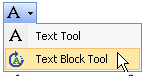
Just as you can move and rotate a shape relative to the page or to a group, you can move a text block relative to a shape! The text block is the conceptual rectangle that holds a shape’s text. It can be moved and rotated independently of the shape. Sitting at the top of the Standard toolbar, just below the big black A is the the Text Block Tool. You have to click the little drop-down triangle to get at it, like this:

Viso Text Block Tool

If you have a copy of Visio with the ribbon, you will find the Text Block Tool in the Tools group on the Home tab. Note: some shapes have protection and guarding that prevents you from doing this, so practice on simple shapes that you yourself have drawn until you get familiar with the tool. Shapesheet junkies will want to know that changes you make with the Text Block tool are reflected in the Text Transform section of the Shapesheet.

F2 Enters Text-edit Mode

It’s easy to select most Visio shapes and simply start typing. But sometimes you want to edit text that is already there, and double-clicking doesn’t always get you into text-edit mode. For these cases, F2 is the shortcut that will get you into text-editing mode. Just select a shape and press F2, and your shape’s text will become highlighted–ready and waiting for you to edit it. Pressing ESC will get you out of text-edit mode.

Setting Double-click to Edit Text

When you draw a simple rectangle or circle, the default double-click behavior is to enter text-edit mode. But if you draw a group, then double-clicking will probably just select one of the group’s sub-shapes. If you have text-heavy drawings with lots of text-containing shapes, you might want to set all shapes so that double-clicking enters text edit mode.

This is really easy to set up if you have an older version of Visio. All you need to do is:

1. Select some shapes 
2. Right-click and choose Format, Behavior, Double-click tab 
3. Check the option button: Edit shape’s text

If you have a copy of Visio with the ribbon then you will have to firstly turn on the Developer tab to locate the Behavior control. Click the File tab and click Options. Under the Customize Ribbon heading, click the Developer tab checkbox to enable your developer tab. Now all you have to do is:

1. Select some shapes
2. Click the Developer tab and the Shape Design group
3. Click the Behavior control
4. Click the Double-click tab
5. Check the option button: Edit shape’s text

In the Shapesheet, an event cell will receive a new formula. It looks like this:

EventDblClick = OPENTEXTWIN()

So if you’re making automation tools that set this behavior automatically, just set the EventDblClick cell!

Process Lists With LOOKUP and INDEX

When you want to work with lists of values on a Visio ShapeSheet use the LOOKUP and INDEX functions to help you out. You often need to know where an item is in a list, or retrieve a specific item from a list. LOOKUP tells you where an item is in a list.

LOOKUP(“three”,”one;two;three;four”) returns 2, as the list positions are zero-based. If the first argument isn’t in the list, the function returns -1. Notice that you can use LOOKUP to do text comparisons too, if you are into code obfuscation.

INDEX returns you the nth item in a list. Again, where n is a zero-based value. So INDEX(1,”one;two;three;four”) returns “two”. By default, the semi-colon is the ShapeSheet’s list-separator of choice, but both functions have optional arguments that let you specify a custom list-separator.

We can demonstrate both functions in a text-translation example. We have two lists of numbers: one in English, one in German. Using LOOKUP and INDEX, we can return the German value from the corresponding English value.

User.numsEN = “zero;one;two;three;four;five;six;seven;eight;nine”
User.numsDE = “null;eins;zwei;drei;vier;fünf;sechs;sieben;acht;neun”
User.valEN = “five” …this could come from ShapeText, or a Shape Data field, for example.

And now we create the calculation formula:
User.valDE = INDEX(LOOKUP(User.valEn, User.numsEN), User.numsDE)

As long as the lists match up, this will work. We get a number that indicates where User.valEN is in the list of English numbers. This index value is then used to return the German equivalent. So: “five” gives us an index of  4, which then points to “fünf”

Resize Font With Shape

ShapeSheeters often ask how to get their text to resize with the shape. Normally, font-size is independent of shape size, but sometimes text should behave less like information and more like graphics. In short, “How do you get font size to change with shape size?”

The easiest way to do this is to create a relationship between the current height of the shape and the original height of the shape, and multiply that by the original font size. The formula can live in the Char.Size cell and might look something like this:

Char.Size = 12pt * Height / 0.75 in 

Here, 12pt is the original font size, and 0.75 in is the original height of the shape. The expression will increase or decrease with the current Height of the shape, and the font size will correspondingly grow or shrink. You might want your text to react with the Width of the shape, or some combination of Height and Width.