Mouse Training London Ltd

Thursday, 16 July 2015

Maintaining Formatting when Refreshing PivotTables

PivotTables provide a great way to analyse large amounts of data and pull out the summarisations that you need. Once you have the PivotTable displaying the values you need, you can then format the table to make the data presentable—for a while.

Note: when you update the data on which the PivotTable is based, after you refresh your PivotTable, your formatting work may go away.

To prevent loss of format when refreshing follow these steps:

Make sure that your PivotTable displays the values you want.
Format the PivotTable to your liking.
From the PivotTable toolbar, select Table Options from the PivotTable menu. The PivotTable Options dialog box opens. (See Figure 1.)

Figure 1. The PivotTable Options dialog box.

Make sure the Preserve Formatting check box is selected.
Click OK.

When you now refresh the PivotTable, your formatting should remain on rows and columns previously applied in the PivotTable.

Note: If the refresh results in new rows being added to the PivotTable, then you will still need to format those, unless you are using an AutoFormat.

PowerPoint- Creating Slides in Outline View

Creating Slides in Outline View

PowerPoint's Outline View is a great way to quickly and easily create slides and bullets. When you start a presentation, the first thing you want to do is to brainstorm all the ideas and topics that you want to cover.

Outline view helps you create your slides and focus on the content and order of your delivery, which is so important to a presentation. You can save the fancy things, like backgrounds, fonts and pictures, for later.

Click on the Outline tab on the left hand side of the Normal view. This switches the normal display of thumbnails to an outline of your presentation. Each icon on the left represents a slide.

Enter and CTRL+Enter to make bullets

To create the slides in a blank presentation, press ENTER. Type in some text and that's the title of your slide. You can create the bullet points on each slide as you go along or you can come back on yourself by doing the slides first and then doing the detailed bullets after.

Pressing ENTER makes a new slide. Pressing CTRL+ENTER indents down to the bullet level. Type in your first bullet then press ENTER to go on to the next one. When you want to do another slide, press CTRL+ENTER.

You can also use TAB and SHIFT+TAB to do the indents and outdents for the outline.

When you want to change the order of your slides, click one of the slide icons (your mouse pointer changes to a four-headed arrow) then drag and drop the slide into a different position.

The slide layouts automatically used for your slides are Title for the first slide and Title and Content thereafter. In Microsoft PowerPoint 2013 the Outline pane has to be turned by clicking the Outline View control in the Presentation Views group on the View tab.

PowerPoint-Balance Diagrams

PowerPoint-Removing backgrounds from Pictures

PowerPoint-Manipulating Text boxes

PowerPoint-Random placeholder text

Thursday, 9 July 2015

Word for Mac- Make your own menu

I like Word for Mac but it makes me feel like a crazy mixed-up kid. I get so confused trying to find things; there's the traditional drop-down menus, there's the toolbar and then there's the ribbon. So many different ways of doing exactly the same thing. Which I wouldn't mind if they were all the same and you just decided which one you preferred to use. But they're not.

Each one is slightly different and some things are on one but not the other and then there's all the things which aren't there at all where you have to know and use the shortcut keys. I can see where they're going with the design and I like it; make Word really easy to use by putting all the everyday things on the ribbon and then tuck the twiddly bits away in the menu. It's just that I get frustrated when I'm trying to get things done.

For example, to work with Word fields you need to be able to update them. The shortcut key is F9. For some fields, like Table of Contents, you don't need F9 because Word gives you a button to click but you do need it for other fields but when you press F9 it doesn't work unless you change the Mac OSX keyboard assignments.

The Word for Mac shortcut keys are essentially the same as the Windows version but usually with Command (⌘) substituted for CTRL. I have to tidy up the formatting on documents quite a lot and one of my favourite key sequences is Select All, Reset Character Formatting and Reset Paragraph Formatting. This brings everything back to the base styles so that you can easily reformat. The shortcut keys are like this:

Command	Windows	Mac
Select All	CTRL+A	Command+A (⌘+A)
Reset Character Formatting	CTRL+Spacebar	Command+SHIFT+Z (⌘+SHIFT+Z)
Reset Paragraph Formatting	CTRL+Q	Command+Option+Q (⌘+⌥+Q)

Guess what? That last one doesn't work on my Mac! I have to change the keyboard assignments because it's nowhere to be seen either in the menu, the toolbars or the ribbon. Either that or it's there and I can't find it. It makes you want to weep. Don't give up, try making your own menu for all the things you need. It's all done with a few clicks and you'll bless yourself.

Making your own Word menu

Have a think about all the Word commands that you tend to use frequently, especially the ones you can never find. They are the ones you need on your menu. Firstly, point to the menu or toolbar, right-click (CTRL+click if you can't do a right click) and click Customize Toolbars and Menus from the end of the shortcut menu.

Step 1. Customize Toolbars and Menus

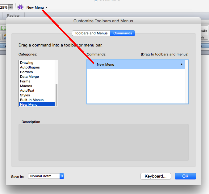
The next thing is to make a new container for your menu. So click on the Commands tab at the top and then look down the Categories list on the left hand side for New Menu. It's right at the end so you will have to scroll down a bit before you can see it.

Step 2. Drag New Menu to a Toolbar or Menu

Now, big decisions to be made. Where shall we put our drop-down menu? You can place it on the Word menubar or a toolbar. Personally, I like to put it on the end of the general toolbar. Click New Menu in the Commands list on the right hand side. As you can see, it's the only one in the list. Drag and drop New Menu to your desired location.

Step 3. Drag items onto your New Menu

For our next trick we need to find the commands for our menu. This can take some time as you have to search for them. Staying with the Customize Toolbars and Menus box, turn your attention back to the Categories list on the left. The categories vaguely follow the main Word application menu so if you know where something is in the menus it should give you a lead as to where to find it in the categories lists. But there's a lot more in the categories list than there is in the menu so be prepared to keep looking. Pretty much every command for Word is listed.

When you have found what you're looking for drag the item out of the list and drop it onto your New Menu. You should see the menu pop-out at you when you hover over it. Click the OK button when you're done.

Step 4. Admire your beautiful New Menu

It's high time to admire the beauty of your new menu. There's all those pesky Word commands that you can never find all gathered together into a nice, easy to use menu. I haven't finished yet, there's a few more Word commands I need on my menu, like Select All and Update Fields. No worries, you can always change your menu anytime you like by clicking Customize Toolbars and Menus again.

Step 5. Choose Properties to rename your New Menu

Should you want to rename your menu just do the right-click thing again and this time click Properties in the shortcut menu. Then just enter some different text into the Name box.

Step 6. Renaming your menu

Word-Selecting Text

Word-No Footers on the Last Page

Word-Using Styles

Word-Typing in Accented Characters

Word-Entering Random Text

Get the Office 2016 Preview for home

Office 365 subscribers

Go to the Office My Account page

Click Language and install options.
Click Additional install options.

Open the Version drop-down menu and select the 32-bit or 64-bit Office 2016 Preview.

This will install the Office 2016 Preview on your device. You will stay on the Office 2016 Preview track until you uninstall the Office 2016 Preview or until Office 2016 is released.

All other Office users

If you don't have an Office 365 subscription, you can download a trial version of Office 2016 Preview from the list of choices below.

Use the product key provided below to activate your trial:

Product key for the Office 2016 Preview

NKGG6-WBPCC-HXWMY-6DQGJ-CPQVG

Download links

Get Office 2016 Preview (32 bit)
Get Office 2016 Preview (64 bit)

Once the trial period expires, you will have the option to purchase an Office 365 subscription or reinstall your current version using your original product key, learn more.

Just remember by loading this up it will remove your existing version of office.

Thursday, 2 July 2015

The Excel Today function

Summer PUBLIC course promotion

£100+VAT, 50% discount on our popular scheduled courses between 1st July – 31st August.

Excel –introduction – intermediate – Advanced – VBA

Word–introduction – intermediate – Advanced

PowerPoint–introduction

Outlook–introduction

Visio–introduction

Additional dates will be added daily.

For latest availability contact course reservations.

This week’s Function and Shortcut Keys

The Excel Today function

returns the current date. The function has no arguments and therefore, the syntax of the function is simply:

TODAY()

Today Function Examples

The following spreadsheets show 2 simple examples of calls to the Today function, which were made on 6th January 2011. The first example shows the function used alone, and the second example shows the function used as a part of a formula that calculates the number of days that have passed since 31-Dec-2009.

The spreadsheet shows the format of the formulas and the spreadsheet on the below shows the results.

Today Function Problem

The following problem is encountered by some people when using the Excel Today function:

Common Problem

When you attempt to subtract another date from the result the Today function, (as in cell B2 of the example above), the result looks like a date (eg. "16/11/1900"), instead of returning an integer.

Possible Reason

This problem arises because the new cell or column is formatted as a 'date'. In this case, it is only the formatting of the cell that is wrong, NOT the value returned by the function.

To correct this:

Highlight the cell(s) with the wrong formatting
Right click with the mouse
Select the Format Cells ... option and ensure the Number tab is selected
Under the Category heading, select the option General and click OK

Selecting Cells

CTRL - Left Mouse Button	-	Selects multiple cells i.e. to select more than one cell (or range), first use the mouse to select on the first cell (or range), then press the CTRL key and use the mouse to select further cells or ranges
SHIFT - Left Mouse Button	-	Selects all cells between (and including) the previous active cell and the cell that is currently being clicked in i.e. to select a range, first use the left mouse key to click on a cell (or row or column) at the start of the range, then press the Shift key and select the cell at the end of the range
SHIFT ↓	-	Moves the current selected range down a row
SHIFT ↑	-	Moves the current selected range up a row
SHIFT →	-	Moves the current selected range right by one column
SHIFT ←	-	Moves the current selected range left by one column
CTRL-SHIFT ↓	-	Selects all cells below the current selection, up to the edge of the current data region
CTRL-SHIFT ↑	-	Selects all cells above the current selection, up to the edge of the current data region
CTRL-SHIFT →	-	Selects all cells to the right of the current selection, up to the edge of the current data region
CTRL-SHIFT ←	-	Selects all cells to the left of the current selection, up to the edge of the current data region
CTRL-Spacebar	-	Selects the whole of the current column(s)
SHIFT-Spacebar	-	Selects the whole of the current row(s)
CTRL-a	-	Selects all cells in the current worksheet

Inputting Data

CTRL - ;

Inserts the current date into a cell

CTRL - :

Inserts the current time into a cell

While in edit mode within a cell, cycles through the 4 different combinations of absolute and relative references :

$A$1

A$1

$A1

Wednesday, 24 June 2015

Selecting Text in Microsoft Word

Still clicking and dragging to select the text in your Word documents? Try these....

Double-click to select a word

Making a single word bold? No problem, just double click to select the word, then click bold. For several words, hold down the CTRL key as you double click the other words.

Double-click to select a word

CTRL click to select a sentence

A sentence is any amount of text between two full stops. CTRL click on any word to select the entire sentence.

CTRL click to select a sentence

Click to select a row

Point at the white space in the left hand margin and click to select the current row. Then drag down to select more rows.

Click to the left to select a row

Double-click to select a paragraph

Again, pointing at the white space in the left hand margin, double-click to select the entire paragraph.

Double-click to select a paragraph

Triple-click to select the whole document

Point at the white space in the left hand margin and triple-click to select all the text in the document. Or press CTRL+A.

Triple-click to select the document

Click twice to position text

Yearning to make a word cloud? Sick of setting tab stops? To easily place text anywhere on the page, just click twice on any place on the page and start typing. Word inserts the paragraph markers and tabs required. That's not a double-click, it's two clicks one after the other.

Click twice to position text

Word-Using Styles

Word-No footers on the Last Page

Word-Typing in Accented Characters

Word-Entering Random Text

Sunday, 11 January 2015

Excel- Protecting the formulas in your worksheet

Lock Cells

You would think that protecting formulas in an Excel worksheet would be easy to do. After all, they are a key element of any worksheet.

The reality is that it can be rather a frustrating process if you don't understand how Excel cell locking and worksheet protection works. It's an old, familiar story; the design dates back to the 1980's when Excel was first released and now it can't be changed because everyone has got used to it. The way you have to do it does seems illogical if you've never done it before. But then if you had done it before you wouldn't need to be reading this article, would you?

So, persevere with this, it does work but you need to suspend common sense and just get on with it. Let's spend a few minutes understanding how worksheet protection and cell locking works and then we can successfully and easily do simple things like protecting our formulas.

How does worksheet protection work?

The theory is that all the cells in an Excel worksheet are locked but the locking is not enabled until you protect the worksheet. You can demonstrate this on a new worksheet if you like.

Click the Format control in the Cells group on the Home tab and then choose Protect Sheet from the menu. Don't worry about entering a password or any of the other options, just click OK and the active sheet is protected. Now, try to type something into a cell, any cell. See, it doesn't happen—you can't make any entries at all.

Protecting the worksheet

All you get is the "The cell that you are trying to change is protected" message box. To turn off the worksheet protection repeat the previous process and choose Unprotect Sheet from the menu.

In practice, protecting the entire worksheet is overkill. You need to be able to make entries in some of the cells and you do this by unlocking them before you turn on the worksheet protection. Remembering, of course, that all cells are locked unless you set them otherwise.

So, the process is that you think about the cells on the worksheet that you wish to be left open for entry and these are the ones which you unlock. Then you protect the worksheet so that only the unlocked cells can be used.

You can not directly select and format a range of cells to be protected. This is what causes the frustration because this is what people expect to be able to do. Well, it can be done but you have to work backwards and it's not a one-step process. What would we do if we had a range of cells on a worksheet that we wanted to protect and we were quite happy that all the other cells would be open for entry?

We would proceed like this:

Select all the worksheet cells and unlock them.
Select the cells you wanted to protect and lock them.
Protect the worksheet.

Quite logical isn't it? Not. But it works. Now, not only is the general method of implementing cell locking and worksheet protection somewhat convoluted but some of the controls in the user interface seem to be designed to promote maximum confusion. Everything we need is in the Protection section of the Format menu.

The process of protecting and unprotecting worksheets is entirely straightforward as the menu has a toggle control which switches between Protect Sheet and Unprotect Sheet. That is a good example of how to design a toggle, the menu caption changes so that you can easily see whether your sheet is protected or not.

However, the process of locking and unlocking cells is not so obvious. Again, we have a toggle control to switch between the two different states but, sadly, the design is not too good as the menu caption does not change at all. Whether you are locking or unlocking your cells the menu caption always reads as Lock Cell.

I am a little disappointed in this as changing a menu caption is the simplest thing to do but by failing to do it the Excel designers have managed to bamboozle and confound countless innocent victims. It's a crying shame. The golden background to the padlock icon is the visual clue—if the padlock has a golden background then the cell is locked and if you click the control you are unlocking the cell.

Now you're going to tell me that the golden background of the icon is not always very distinct against the golden background of the active selection. And I am going to agree with you because the menu caption should really switch between Lock Cell and Unlock Cell just as the sheet protection setting does. But it doesn't. Sorry. I hope that this all made sense.

Selecting and Protecting Formulas

If you want to protect the formulas in your worksheet then you will need to be able to select your formulas easily without having to do it yourself. Click the Find & Select control on the extreme right hand side of the Home tab and choose Formulas from the menu.

Selecting formulas

All the formulas in the entire active worksheet are now selected. If you select a range first then only those cells containing formulas inside your current selection are selected.

Here is the step-by-step process for protecting all the formulas in the entire worksheet:

Select all the cells.
Unlock all the cells.
Select the formula cells.
Lock the formula cells.
Protect the worksheet.

It does seem rather a rigmarole but once you've done it a few times it's easy to remember. Each worksheet has to be done individually. You can always automate the entire process by recording a macro. Watch out for my future article where we shall record a macro to protect a single worksheet and then adapt it so that all of the worksheets in the workbook are protected.

If you want your documents to be secure then you should definitely consider entering a password when you protect your worksheet otherwise the worksheet protection can be easily turned off by anyone.

Here's the five steps in detail:

1. Select all the cells

Click the keystone at the intersection of the first row and the first column or press CTRL+A.

2. Unlock all the cells

Click Home tab, Cells group, Format control and choose Lock Cell (yes, really!) from the menu.

3. Select the formula cells

Click Home tab, Editing group, Find & Select control and choose Formulas from the menu.

4. Lock the formula cells

Click Home tab, Cells group, Format control and choose Lock Cell from the menu.

5. Protect the worksheet

Click Home tab, Cells group, Format control and choose Protect Sheet from the menu.

Excel-Make Pivot Tables refresh automatically

Excel-Calculations without formulas

Excel-Sorting by last name

Excel-Switching columns to rows

Excel-CTRL key tricks

Excel-Double click tricks

Excel-Converting USA dates to UK dates

Excel Top ten shortcut keys

Excel 2010 shortcut keys

Excel-AutoSum Revisited

Excel for Mac-Deleting a range and other shortcuts

Tuesday, 9 December 2014

Excel- The Countdown to Christmas

Have you ever wondered how many shopping days are left until Christmas or what day of the week is Boxing day? How many days until payday? Or which day of the week is my birthday? Maybe you're forever asking yourself am I Wednesday's child or Friday's child?

Hurl your diary away, spurn your smartphone, ignore your fingers and turn to Excel for the answers to all these date conundrums. All Excel dates are stored as numbers and a few simple formulas and functions combined with a passing knowledge of date format codes is all you will ever need. Just make sure that you type-in your dates correctly otherwise you won't be able to use them in your calculations and your date formats won't work.

Entering Dates

Whenever you type a date into an Excel cell remember to use slash or dash separators like this: 9/12/14 or like this 9-12-14. It's years since we had to worry about the Millennium bug but if you're feeling fussy or you need a date in the last century then use 4 digits for the year i.e. 9/12/2014. Simply type-in the day and month and Excel presumes that it's the current calendar year so entries like this 9/12 or 9-12 will suffice. Please don't use dot separators like this, 9.12.2014. They won't work unless you first change your Windows Control Panel settings.

The main thing is to make sure that the entry you make evaluates properly to a date and the best visual check is to see whether your date aligns to the right hand side of the cell but its always worth checking in the formula bar to see whether your date looks like this, 09/12/2014. When a cell contains a date you can make the date appear however you like by applying a date format.

How many shopping days to Christmas?

I am going to presume that you will be able to shop on a Sunday but you will not want to venture forth on Christmas day itself so we need to work out the number of days between today and the 24th December.

Not long to go!

We want our calculation to show the number of dates automatically as time passes so rather than type-in today's date as a constant it is best to use Excel's TODAY function which always returns the current date.

In the illustration 24/12/2014 is entered into cell A1 and the formula =TODAY( ) is entered into cell A2. Don't forget the brackets for the function, nothing is required inside them but they have to be there for Excel to recognise the function call.

When you make your entry you only need type the first, opening bracket, the formula is not case sensitive so it is quite acceptable to just type-in "=today(". The final job is to calculate the difference in days between the two dates, for this we enter a simple formula in another cell to minus the earlier date from the later date, in cell A3 the formula is =A1-A2.

Come back tomorrow, the difference will one day less and you still haven't done your cards. Have you?

What day of the week is Boxing Day?

Now, I'm quite a sharp fellow and I know that Boxing day is the 26th December, the day after Christmas day. I even used to know why it is called Boxing day but what I don't know is what day of the week it is. No problem. Firstly enter 26/12/2014 into a convenient cell, then right-click and choose Format Cells from the shortcut menu. Click the Number tab and then Custom at the end of the category list. Don't go to the Date category as Excel does not have a standard format to show the day of the week, instead we are going to create one.

Formatting dates using a Custom Number format code

Date Format Codes

Excel date format codes are made up of combinations of d, m and y codes for day, month and year values using as many or as few as you need. For example, d gives you today's date as significant digits (1 as 1, 26 as 26), dd gives you today's date as two digits (1 as 01, 26 as 26), ddd gives you the short day of the week i.e. Fri and dddd gives you the full day of the week i.e. Friday.

Use the existing date codes as a pattern and examine the results of your format code in the Sample box as you type the code elements into the Type box. You can always re-use any format codes that you have already created in this workbook—they are stored at the end of the Custom list.

Enter your dddd code, click OK and now your cell shows that, this year, Boxing day is on Friday.

The Excel Christmas Date Challenge

For your homework tonight you have to:

Assuming you've already received your December salary and blown it. Calculate how many days you have to survive until your next pay day on 30th January 2015.
Work out on which day of the week you were born.

Remember that it goes like this:

Monday's child is fair of face,
Tuesday's child is full of grace,
Wednesday's child is full of woe,
Thursday's child has far to go,
Friday's child is loving and giving,
Saturday's child works hard for a living,
And the child that is born on the Sabbath day is bonny and blithe, and good, and gay.

Does the old rhyme work for you? I was born on a Friday and while I have been called many things I don't remember it ever being loving or giving.

Excel-Tick marks and Check boxes in cells