Excel Text Function

Microsoft Excel Text Function

Basic Description

 

The Excel TEXT function converts a supplied value into text, in a user-specified format.

The format of the function is :

TEXT( value, format_text )

Where the function arguments are:

value	-	A numeric value, that you want to be converted into text
format_text	-	A text string that defines the formatting that you want to be applied to the supplied value

The format definitions that can be used in the Excel Text function are shown in the table below. These definitions have the same meaning when used in the custom style of Excel Cell Formatting.

0	-	Forces the display of a digit in its place
#	-	Display digit if it adds to the accuracy of the number (but don't display if a leading zero or a zero at the end of a decimal)
.	-	Defines the position that the decimal place takes
d	-	Day of the month or day of week d = one or two digit representation (eg. 1, 12) dd = 2 digit representation (eg. 01, 12) ddd = abbreviated day of week (eg. Mon, Tue) dddd = full name of day of week (eg. Monday, Tuesday)
m	-	Month (when used as part of a date) m = one or two digit representation (eg. 1, 12) mm = two digit representation (eg. 01, 12) mmm = abbreviated month name (eg. Jan, Dec) mmmm = full name of month (eg. January, December)
y	-	Year yy = 2-digit representation of year(eg. 99, 08) yyyy = 4-digit representation of year(eg. 1999, 2008)
h	-	Hour h = one or two digit representation (eg. 1, 20) h = two digit representation (eg. 01, 20)
m	-	Minute (when used as a part of a time) m = one or two digit representation (eg. 1, 55) m = two digit representation (eg. 01, 55)
s	-	Second s = one or two digit representation (eg. 1, 45) ss = two digit representation (eg. 01, 45)
AM/PM	-	Indicates that a time should be represented using a 12-hour clock, followed by "AM" or "PM"

Problem with Simple Concatenation of Dates

Because an Excel date is stored as a simple number in Excel, if you attempt to join a name and date into a text string by just using the simple & operator, this will be displayed as a name followed by a number.

For example, if used in cell C2 of the spreadsheet below, the formula:

=A2 & " " & B2

gives the following result:

 

Text Function Example 1

One of my most common uses of the Excel Text function is to insert dates into text strings.

Without the use of the Text function, the simple concatenation of a text string with a date gives an unexpected result (see right).

The spreadsheet below shows the Excel Text function used to produce the required merged text string.

As shown in the formula bar, the formula used is:

=A2 & " " & TEXT( B2, "dd/mm/yyyy" )

Text Function Example 2

The examples below show use the Text function, with a variety of specified formats. The spreadsheet on the left shows the function formats and the spreadsheet on the right shows the results.

Formulas:

Results:

Note that the results of the Text function, in column B of the spreadsheet above, are all text values, rather than numeric values.

Further information and examples of the Excel Text function can be found on the Microsoft Office website.

Excel Text Function Error

Some users have problems when the Excel Text function returns the #NAME? error:

Common Error

#NAME?

-

This is returned from the Excel Text function, if you omit the quotation marks from around the format_text For example, the formula =TEXT( A2, dd/mm/yyyy ) will return the #NAME? error. Solution:   Add quotes around the formatting definition. Eg. the above example would be corrected as: =TEXT( A2, "dd/mm/yyyy" )

Excel Fixed Function

Microsoft Excel Fixed Function

Basic Description

 

The Excel FIXED function rounds a supplied number to a specified number of decimal places and then converts this into text.

The format of the function is :

FIXED( number, [decimals], [no_commas] )

Where the arguments are as follows :

number	-	The number to be converted into a text string
[decimals]	-	An optional numerical argument which specifies the number of decimal places to be shown after the decimal point Note : - If [decimals] is omitted, it takes on the default value of 2 - If [decimals] is negative, the supplied number is rounded up to the left of the decimal point - If [decimals is a decimal (rather than an integer), it is truncated to an integer
[no_commas]	-	An optional logical argument which specifies if the returned text should separate thousands by commas. Possible values are : TRUE - Commas are not included in the resulting text FALSE - Commas are included in the resulting text If the [no_commas] argument is omitted, it takes on the default value of FALSE.

Fixed Function Examples

The spreadsheet below shows examples of use of the Excel Fixed Function. The spreadsheet on the left shows the format of the functions and the spreadsheet on the right shows the results.

Formulas:

Results:

Fixed Function Common Problem

Common Problem

Once a number has been converted, using the Excel Fixed function, it is stored in Excel as text. Therefore, it cannot be used in numeric calculations. 

If you want to be able to use the numbers in calculations, you may prefer to keep the values as numbers in Excel and just change the formatting into the required numeric format. To do this:

• Right click with the mouse, on the cell to be formatted
• Select the Format Cells ... option and ensure the Number tab is selected
• Under the Category heading, select the option Number
• From the options that appear on the right, specify the details of the formatting required
• Click OK

Excel Dollar Function

Microsoft Excel Code Function

Basic Description

The Excel DOLLAR function rounds a supplied number to a specified number of decimal places and then converts this into text, using a currency format. The currency format used is the format that is set as the default on your computer.

The format of the Excel DOLLAR function is :

DOLLAR( number, [decimals] )

Where the arguments are as follows :

number	-	The number to be converted into a text string
[decimals]	-	An optional numerical argument which specifies the number of decimal places to be shown after the decimal point Note : -     If [decimals] is omitted, it takes on the default value of 2. -     If [decimals] is negative, the supplied number is rounded up to the left of the decimal point.

Dollar Function Examples

Formulas: A B 1 =DOLLAR( 123.591 ) 2 123.591 =DOLLAR( A2 ) 3 123.591 =DOLLAR( A3, 1 ) 4 123.591 =DOLLAR( A4, 0 ) 5 123.591 =DOLLAR( A5, -1 ) 6 123.591 =DOLLAR( A6, -2 )

Results: A B 1 $123.59           2 123.591 $123.59 3 123.591 $123.6 4 123.591 $124 5 123.591 $120 6 123.591 $100

Dollar Function Common Problem

Common Problem

Once a number has been converted, using the Excel Dollar function, it is stored in Excel as text. Therefore, it cannot be used in numeric calculations.

If you want to be able to use the numbers in calculations, you may prefer to keep the values as numbers in Excel and just change the formatting into a currency format. To do this:

• Right click with the mouse, on the cell to be formatted
• Select the Format Cells ... option and ensure the Number tab is selected
• Under the Category heading, select the option Currency
• From the options that appear on the right, specify the details of the formatting required
• Click OK

Excel Bahttext Function

Microsoft Excel Bahttext Function

Basic Description

The Excel Bahttext function converts a number into Thai text, with the the suffix "Baht".

The syntax of the function is :

BAHTTEXT( number )

Where the number argument can be supplied to the function either directly, or as a reference to a cell containing a number.

Bahttext Function Examples

The following spreadsheet shows two simple examples of the Excel Bahttext function. The format of the function is shown in the spreadsheet on the left and the result is shown in the spreadsheet on the right.

Formulas:

Results:

 

Bahttext Function Error

If you get an error from the Excel Bahttext function, this is likely to be the #VALUE! error :

#VALUE!

-

Occurs if the supplied number argument is not recognised as a numeric value.

Excel Trim Function

Microsoft Excel Trim Function

Basic Description

 

The Excel Trim function takes a supplied text string and removes any spaces, except for single spaces between words or characters.

The syntax of the function is :

TRIM( text )

where the 'text' argument can be supplied to the function either directly, as a text string returned from another formula, or a reference to a cell containing text.

Note that the Trim function differs from the Clean Function in that the Trim function removes additional spaces (represented by the ASCII numeric code 32), while the Clean Function removes the non-printable characters, represented by the ASCII numerics codes 0 to 31.

Trim Function Examples

The example below shows the Trim function used on four different text strings.

In all four of the above cases, the result is the string

"trimmed text"

- with no spaces at the start or end and just one space in the middle.

Excel Clean Function

Microsoft Excel Clean Function

Basic Description

The Excel CLEAN function takes a supplied text string and removes all non-printable characters.

The function is designed to remove the non-printable characters, represented by numbers 0 to 31 of the 7-bit ASCII code, which are often found at the start of data that has been imported into Excel from other applications.

The syntax of the function is :

CLEAN( text )

where the 'text' argument can be supplied to the function either directly, as a text string returned from another formula, or a reference to a cell containing text.

Clean Function Examples

The example below shows the Excel Clean function used on four different text strings.

All four of the above examples give the same result, which is the string,

"clean text"

Creating a New Microsoft Access Database

Creating a New Microsoft Access Database  

A new Access file is an empty database that you create or it may be based on an existing
template where certain elements of the database are created automatically.

When you create a new database, it has to be saved. Whereas when you create a new
document in Word or a new spreadsheet in Excel, you can set up the document or
spreadsheet and then decide when to save.

The Process to create a database is

• Click on the Office button.

• Select New.

(Using the Office button is not necessary if you are creating a new database on first entering
Access).
.

A New Blank Database

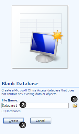
 To create a blank database click on Blank Database  This will then allow you to name and save the database into a chosen location


1. Click on the button and choose the  location of the database.

2. Enter the file name for the database.

3. Click on the create button.

  

A New Database From a Template

1. When a new database is going to be based on a template, you need access to where the
template is. The database template can be on your machine or it can be a Microsoft
template that you need to connect to on-line.

2. Once a template category has been selected, it updates the list of templates available.
Select the template required.

3. A database with the same name as the template will be created and saved in the default
location unless you choose the location and give the database a name.

File names can be upto 255 characters (including the file extension) the name cannot start
with a space but can have spaces within the name. Ccertain characters should not be used
in file names as they can produce unexpected results. These are invalid characters for file
names ?, ",/,\,<,>,|,:
When a new database is created any database that was already open will automatically be
closed. If anything needed to be saved a prompt would have come up asking you to save if

you wanted to.
Microsoft Access can only have one database open at a time. The same is true when you
open an existing database. If you want more than one database open at the same time then
you need to have Microsoft Access running once for each database.

Microsoft Access Column Views

Microsoft Access Column Views 

At times, you do not want to view the table in a particular way.
Sometimes there will be columns that you do not want to see as they are not relevant at that
point in time for what you need.
At other times as you scroll across to view other columns you still want to be able to see key
columns.
Hiding/hiding columns

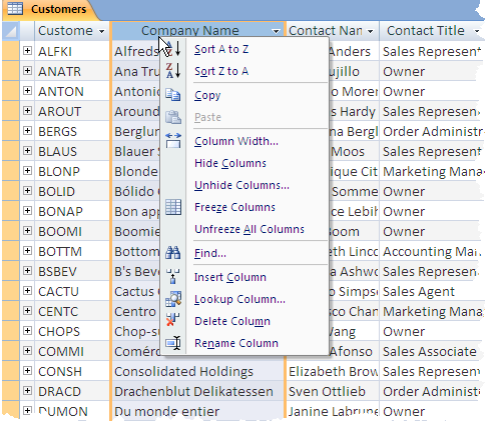
Columns can be hidden by
1. Highlight column(s).
2. Right click on column heading of column to be hidden.
3. Select Hide columns.


Columns can be unhidden by
Highlight column(s) on either side of the hidden column(s)
1. Right click on column heading.
2. Select Unhide Columns.

Freezing Columns

At times as you scroll across the
screen, you want to be able to
always see certain columns rather
than have them disappear to the left
so that you can identify the records.
In this example, we can see the city
country and telephone numbers but
we can’t tell who the customers are.

Columns can be frozen by:

1. Highlight columns to be
frozen.
2. Right click on column heading
3. Select Freeze Columns.
(Frozen Columns can be
unfrozen by selecting the
Unfreeze All Columns command).



By freezing customer id and
customer name columns as you
scroll across to see other data
you will still see the two frozen
columns.

Excel- Tick Marks and Check Boxes in cells

Check boxes, a pipe-dream?

It isn't much to ask for is it? Cells with tick marks (or check boxes if you like) would tick all the boxes for me. After all, you can easily create Yes/No fields in Microsoft Access tables and creating check boxes in Apple Numbers is a breeze but poor old Excel just doesn't seem to want to play the check box game.

Yes, you can draw Form Controls or ActiveX Controls on a worksheet and link them to the cells but it is such a long-winded and painful process when you need loads of check boxes. I want an entire column full of check boxes, I want them in the cell and not on the cell and I want to do them quickly and easily. Dream on.

Rant over, the awful truth is that if the Excel designers don't give you exactly what you want then you have to do it yourself and here's how to do a home-brew version of an Excel in-the-cell checkbox. It involves doing an Excel macro and creating a shortcut for it but don't let that put you off as it only takes a few minutes and then you can have as many check boxes or tick marks as you like whenever you like.

Step One. Record a Macro

You need a module to store your macro and the easiest way to get one is to turn on the macro recorder and then turn it off again. Click Record Macro in the Macros control on the View tab.

Recording a macro

When this dialog displays, enter the Macro name. This one is named as "TickToggle" but you can name it as you like (no spaces are allowed in macro names) Set the shortcut key by typing a letter into the Shortcut key box. I am using the letter "t" (t for ticks!) Try not to use a shortcut key that you want to keep for other purposes, like maybe CTRL+C.

The final setting is to drop the list for Store macro in and select Personal Macro Workbook. Click the OK button, click a cell on your worksheet and then click Stop Recording in the Macros control on the View tab.

Step Two. Copy and Paste the Tick Mark code

Now the macro has been recorded you need to find it and substitute the recorded macro with the macro code that does the tick marks.

Unhiding PERSONAL

The Personal Macro Workbook is a hidden document so we need to unhide it first. Click the Unhide control in the Window group on the View tab and choose PERSONAL from the list.

Then we need to see the code of the recorded macro. Click View Macros in the Macros control on the View tab, select "TickToggle" in the listing and then click the Edit button on the right hand side.

This will transfer you to the macro editor and your screen should be looking something like the illustration below.

The recorded macro

Don't worry if it's not exactly the same so long as you have the first and last lines the same. Everything between the Sub and End Sub lines will be replaced.

The final part of this step is to copy and paste our new tick mark macro, save the file and exit from the editor.




Here's the macro code to copy and paste:

Sub TickToggle()

    On Error Resume Next

    If ActiveCell = "" Then
        With ActiveCell
            .Formula = "=CHAR(252)"
            .Font.Name = "Wingdings"
        End With
    Else
        ActiveCell.Clear
    End If

End Sub

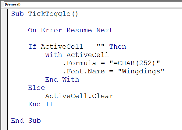
The finished macro

Here's the macro in the editor after the above code has been pasted. Translating the code into plain English, it reads as follows "If the cell is empty then enter character 252 into the cell and set the font format as Wingdings, otherwise clear the cell". Character 252 in Wingdings is a tick mark.

Choose File, Save in the menu and then exit from the editor and return to Excel by choosing File, Close. When you're back in Excel click the Hide control in the Window group on the View tab to hide PERSONAL.

Step Three. Test the macro

Click a cell, press your shortcut keys CTRL+t and a tick mark appears in the cell, press them again and the tick mark disappears.

Tick marks!

Centre-align the cell if you want your ticks centred and change the column width setting.

Your macro is stored in your Personal Macro Workbook which opens automatically when you start Excel and you can use this macro on any workbook. See the next section if you prefer check boxes to tick marks.

Ticks or Boxes?

There's a big decision to make here; do you want to have a tick in the cell and then an empty cell when you turn it off or do you want a proper check box with a tick in it which then changes to an empty box when you turn it off?

The macro above is the "plain tick or an empty cell" version, if you want the "ticked box or un-ticked box" version then you need to change the macro code so that the correct character is entered into the cell. The plain tick is Wingdings character 252, the ticked check box is character 254 and the un-ticked box is character 168. Change your macro by copying and pasting the code below. 

The logic required is slightly different, now it reads in plain English as "If the cell is empty or if it contains character 168 (an un-ticked box) then enter character 254 (a ticked box), otherwise enter character 168".

Copy and Paste this macro for check boxes

Sub TickToggle()

    On Error Resume Next

    If ActiveCell = "" Or ActiveCell.Formula = "=CHAR(168)" Then
        With ActiveCell
            .Formula = "=CHAR(254)"
            .Font.Name = "Wingdings"
        End With
    Else
        With ActiveCell
            .Formula = "=CHAR(168)"
            .Font.Name = "Wingdings"
        End With
    End If
 
End Sub

Checking if the cell has been ticked

If all you need is a simple tick or checkbox in the cell then you're fine but what if you have to have a formula or some Conditional Formatting in the worksheet do something as a result of the cell being ticked or the box checked?

Usually you would use a formula to make a logical test giving you TRUE or FALSE so that you could do something to respond to the current state of the check box. Here's the sort of logical constructions that can make the relevant tests:

Check Tests

Checking for the tick-mark or empty cell is the easiest one as all you are doing is asking "is the cell empty?", which can be done like this:

=ISBLANK(A1)

Where A1 is the cell containing the tick. ISBLANK returns FALSE if the cell contains a tick. Should you find the test easier to process if you return TRUE for a ticked cell then reverse the logic as follows:

=NOT(ISBLANK(A1))

The check box is a little harder as you asking "does the cell contain character 254?" (a ticked box) and you have to use Excel's CELL function as follows:

=CELL("contents",A1)=CHAR(254)

Happy ticking...

Related Posts

Excel-Calculating age from date of birth

Excel-Calculations without formulas

Excel-Sorting by last name

Excel-Switching columns to rows

Excel-CTRL key tricks

Excel-Double click tricks

Excel-Converting USA dates to UK dates

Excel Top ten shortcut keys

Excel 2010 shortcut keys

Excel-AutoSum Revisited

Excel for Mac-Deleting a range and other shortcuts

Excel-Make Pivot Tables Refresh automatically

Training Courses

If you've still got that "I just don't know what I'm doing" feeling then you might like to arrange an Excel training course for yourself or with some of your colleagues. It's really easy to book one of our courses and they're great value for money. See our website for full details.

Apple OS X Yosemite Preview

Yosemite is Apple's next big release of their desktop operating system due out later this year. Once again, as a free upgrade for existing Mac owners. 

Apple has better integrated its desktop OS with their iPhone and iPad iOS 7 devices. While the look of the desktop matches the iOS 7 interface design with translucency, brighter, flatter styling, new icons and fonts mercifully they've not had a Windows 8 moment; it's still a traditional desktop with drop down menus and a dock.

Phone You can make and receive phone calls on your Mac. When your iPhone rings, the caller's name, number and picture show as a notification on your Mac. You can answer calls by clicking the notification and your Mac becomes a speakerphone. You can make phone calls using Contacts, Calendar, Messages and Safari.

No WiFi? Your Mac automatically uses the personal hotspot on your iPhone which appears in the Mac's WiFi menu.

Messages All the SMS and MMS messages that you receive on your iPhone now appear in Messages regardless of what type of phone your friends and colleagues are using. You can respond using whichever device is the most convenient.

iCloud Drive You can store any file in your iCloud Drive and then find it on any device. The iCloud Drive is available in the Finder window and works like any other folder on your Mac, just drag and drop your files into the folder. You can rearrange everything as you wish and see all your files organised in the same way on your iPhone and iPad.

Mail Drop You can send large attachments without having to worry whether they will get through or not. Send large files like videos, images and presentations and they are automatically uploaded to iCloud. Mail Drop works with any email service, if your recipient uses Apple Mail then they receive the attachment as they normally do, otherwise they receive a link to download the file.

AirDrop Sharing files is so easy with AirDrop, you can take a file from any folder and send it to a nearby Mac or iOS device and vice versa. Send a document to a colleague in the next room or send a presentation to a customer across the table. Easy.

Handoff You can automatically pass whatever you're doing from one device to another whenever they are in range. Start writing an email on your iPhone and then finish typing it on your Mac using a full keyboard without losing your place. Or start writing a report on your Mac and finish it off on your iPad on the train home. Handoff works with the following apps: Mail, Pages, Numbers, Keynote, Maps, Messages, Reminders, Calendar, Contacts and Safari.

See more on the Apple website

Excel-the Highest and the Lowest. MIN, MAX, SMALL and LARGE.

Entering Excel's LARGE function

Most people know about the MIN and MAX worksheet functions to calculate the highest and lowest values in a range.

But what about the ninth highest or the third lowest? That's where you need the functions LARGE and SMALL.

The LARGE function

In the illustration above we have a list of countries in column B and a corresponding list of numbers in column C. The formula to calculate the ninth highest number in column C is:

=LARGE(C:C,9)

If you then wanted to identify which country in column B that number referred to you would firstly have to find out where the number was in column C and then use that information to refer back to column B. Use the MATCH function to locate the ninth highest number in column C and then the INDEX function to look up the country from column B.

The formula for the match is as follows (presuming the LARGE formula is entered into cell E4):

=MATCH(E4,C:C,0)

The match formula gives a number that locates the value in column C and then you use that number to index column B (presuming that the MATCH formula is entered into cell E6):

=INDEX(B:B,E6)

Of course, you don't have to do three separate formulas, you can combine LARGE and MATCH into one formula like this:

=MATCH(LARGE(C:C,9),C:C,0)

Or do the entire calculation in one like this:

=INDEX(B:B,MATCH(LARGE(C:C,9),C:C,0))

The SMALL function

The SMALL function is much the same as LARGE, for example =SMALL(C:C,3) gives you the third smallest value in column C:C.

The MIN and MAX functions

=SMALL(C:C,1) will give you the lowest value in column C but it's much easier to use the MIN function to calculate the lowest value in a range. =MIN(C:C) gives the lowest value in the column C, similarly, =MAX(C:C) gives the highest value.

Related Posts

Excel-Calculating age from date of birth

Excel-Calculations without formulas

Excel-Sorting by last name

Excel-Switching columns to rows

Excel-CTRL key tricks

Excel-Double click tricks

Excel-Converting USA dates to UK dates

Excel Top ten shortcut keys

Excel 2010 shortcut keys

Excel-AutoSum Revisited

Excel for Mac-Deleting a range and other shortcuts

Excel-Make Pivot Tables Refresh automatically

Training Courses

If you've still got that "I just don't know what I'm doing" feeling then you might like to arrange an Excel training course for yourself or with some of your colleagues. It's really easy to book one of our courses and they're great value for money. See our website for full details.

Excel- Roman Numerals

Use Excel's ROMAN function if you need to express normal, arabic numbers as Roman numerals.

Excel's ROMAN function

Just type "=r" into a cell and you will see a list of Excel functions pop up, then double-click ROMAN in the list to start your formula. If you like using the keyboard then type-in "=ro" and press the TAB key.

Enter the reference of the cell containing the number you want converted and you're done. Excel's ROMAN function converts positive numbers up to a maximum of 3999. The optional Form argument gives you a choice of up to four degrees of simplification of the classic roman form. For example, the value of 2500 can not be simplified and is expressed as roman MMD. However, 2499 is MMCDXCIX in the classic form but MMID in the simplified form. 

Enter your formula as =ROMAN(E6,FALSE) for the simplified form or use a number from 1 to 3 for the less simplified forms, i.e. =ROMAN(E6,2) gives you MMXDIX. I'm glad we don't have to use roman numerals in our Excel worksheets, no wonder Maximus* was always in a bad mood. 

Excel's 2013 ARABIC function

If you've got a copy of Excel 2013 you can convert roman numerals to arabic using the ARABIC function which was introduced with this version.

"My name is Maximus Decimus Meridius, commander of the Armies of the North, General of the Felix Legions, loyal servant to the true emperor, Marcus Aurelius. Father to a murdered son, husband to a murdered wife. And I will have my vengeance, in this life or the next."

*Sorry, I just had to.

Related Posts

Excel-Calculating age from date of birth

Excel-Calculations without formulas

Excel-Sorting by last name

Excel-Switching columns to rows

Excel-CTRL key tricks

Excel-Double click tricks

Excel-Converting USA dates to UK dates

Excel Top ten shortcut keys

Excel 2010 shortcut keys

Excel-AutoSum Revisited

Excel for Mac-Deleting a range and other shortcuts

Excel-Make Pivot Tables Refresh automatically

Training Courses

If you've still got that "I just don't know what I'm doing" feeling then you might like to arrange an Excel training course for yourself or with some of your colleagues. It's really easy to book one of our courses and they're great value for money. See our website for full details.

Microsoft Project Top Ten Tips

A new departure this week, the first in our series of Hints and Tips for Microsoft Project. Except where indicated, all these tips work with every version of Microsoft Project.

1. To hide a column in a Gantt Chart Table or indeed any table, click the right hand edge of the column header and drag it over to the left until it disappears from view. It is now a zero width column. To display the column, click to the right of the column separator bar where the column used to be. Then drag over to the right. 


2. To link or unlink tasks that are not on consecutive rows, click on one task then hold down the CTRL key and click on another task. Hold down the key to select other tasks. 


3. To change information for a number of tasks at once, select the tasks (use the method described above for non-adjacent tasks) and click the Task Information button. Enter the common information in one of the fields displayed in the Multiple Task Information dialog box.


4. If a task does not reschedule when it is based on a dependency, it may because it contains a "fixed" date of some kind. A fixed date could be an Actual Start or a constraint such as Must Start On or Start No Earlier Than. Use the Tasks with Fixed Dates Filter to view only those tasks in a plan that contain fixed dates. You can then determine if these tasks should have these types of fixed dates. 


5. Press ALT+Home in the Gantt chart to position the chart on the start of the project.


6. Use the INSERT key on your keyboard to insert rows and columns. In the Gantt chart, click on a row and press the INSERT key to insert a blank row above the selected row. Click on a column header to highlight a column and press INSERT to insert a column to the left of the selected column. 


7. To move multiple task boxes in the Network Diagram (PERT Chart) select any number of boxes and then click on the border of a box and drag the entire selection of boxes to a new location. In Project 2000, 2002 and 2003 you must first choose the Format menu, Layout and then Manual Box Positioning to enable this action.


8. In Project 2000, 2002 and 2003, to prevent an item from appearing in the legend for the Gantt chart, choose the Format menu, Bar Styles and place an asterisk (*) before the name of the item that you do not want to appear.


9. To split the screen and place a specific View into the lower pane, hold down the SHIFT key when selecting an item from the View menu. You can also split the screen by selecting Split from the Window menu or doubleclick the small horizontal split bar in the lower right corner of the screen. Double click again to remove the split (or choose Remove Split from the Windows menu).


10. To change the field in a column, double click on the column header and select the new field from the Field Name list. While in the Field Name list, press the first letter of the desired field to go to that field.

Excel- Automatically change the Pivot Table source data range

When you change the source data of a Pivot Table you need to Refresh to reflect these changes but if you add any new rows to the end or columns to the sides of the list, refreshing the data does not detect these additions to the original source data range unless you converted your original range to a Table and then used the Table as the source data  for your Pivot Table.

If you used the original range as your data source then you will have to update the definition of the Data Source by clicking the Change Data Source control on the Options tab of PivotTable Tools. And you will have to repeat this process every time you add any new rows to your list.

Changing the Data Source range automatically

We saw in an earlier article, Make Pivot Tables refresh automatically how to refresh a Pivot Table automatically using the Worksheet_Activate event.

You can change the Worksheet_Activate macro so that in addition to refreshing the Pivot Table it also updates the definition of the Data Source. Thus the Pivot Table responds to any additions or deletions made to the original data range. Copy and paste the section below into your Worksheet_Activate macro:

---

Private Sub Worksheet_Activate()
    Dim PTRange As Range

    'Reset the data source.
    Set PTRange = Sheets("Sheet1").Range("A1").CurrentRegion

    ActiveSheet.PivotTables("PivotTable2").ChangePivotCache ActiveWorkbook. _
        PivotCaches.Create(SourceType:=xlDatabase, SourceData:= _
        PTRange, _
        Version:=xlPivotTableVersion10)
 
    'Refresh PT.
    ActiveSheet.PivotTables("PivotTable2").PivotCache.Refresh

End Sub

---

You need to be a wee bit careful with the macro above and check the following:

• The example assumes that your Pivot Table source data range is on "Sheet1" of the workbook and is a range that starts with cell reference "A1". Should this not be the case then you must change the following line as required:
"Set PTRange = Sheets("Sheet1").Range("A1").CurrentRegion"

• The example assumes that your Pivot Table is "PivotTable2". To find out the name of a specific Pivot Table, right-click one of its cells and choose Pivot Table Options from the short cut menu.

Visual confirmation

If you want to visually confirm that your Pivot Table has been refreshed you can place an unobtrusive message down the bottom of the Excel window on the Status Bar. Add the following line to your Worksheet_Activate macro and clear the message away when you activate a different sheet using the Worksheet_Deactivate event.

---

Private Sub Worksheet_Activate()
 
    'The updating & refreshing macro goes here…...see above
 
    'Show message.
    Application.StatusBar = "Pivot Tables updated at " & Time

End Sub

---

Private Sub Worksheet_Deactivate()
 
    'Clear message.
    Application.StatusBar = False

End Sub

---

Excel's Status Bar

Excel's Status Bar is visible at the bottom of the Excel window and your messages are always shown on the left hand side. If you don't want the time stamp shown in your message then leave out the "& Time" part of the message.

Related Posts

Excel-Calculations without formulas

Excel-Sorting by last name

Excel-Switching columns to rows

Excel-CTRL key tricks

Excel-Double click tricks

Excel-Converting USA dates to UK dates

Excel Top ten shortcut keys

Excel 2010 shortcut keys

Excel-AutoSum Revisited

Excel for Mac-Deleting a range and other shortcuts

Excel-Calculating age from date of birth

Training Courses

If you want to find out more about Excel Pivot Tables or Macros then you might like to arrange an Excel training course for yourself or with some of your colleagues. It's really easy to book one of our courses and they're great value for money. See our website for full details.

Excel- Make Pivot Tables Refresh Automatically

This post has now moved to our new site 

Related Posts

Excel-Calculations without formulas

Excel-Sorting by last name

Excel-Switching columns to rows

Excel-CTRL key tricks

Excel-Double click tricks

Excel-Converting USA dates to UK dates

Excel Top ten shortcut keys

Excel 2010 shortcut keys

Excel-AutoSum Revisited

Excel for Mac-Deleting a range and other shortcuts

Excel-Calculating age from date of birth

Training Courses

If you want to find out more about Excel Pivot Tables or Macros then you might like to arrange an Excel training course for yourself or with some of your colleagues. It's really easy to book one of our courses and they're great value for money. See our website for full details.

Excel for Mac - Deleting a range and other shortcuts

Excel for Mac

Deleting a range of cells in an Excel worksheet is easy isn't it? Surely you just press the Delete key? Well, if you've ever tried it in Excel for Mac then you know a lot better than that. Because deleting a range of cells is a most irritating business as the Delete key doesn't seem to work properly.

Most of us just resort to the main menu and choose Edit, Clear, Contents and either shrug in dumb resignation or weep bitter tears of frustration. Are we missing something? Yes, that's because it's fn+Delete to clear a range of cells. Microsoft Excel for Mac was released in 1985, well before the Windows version. It should be the daddy but I'm afraid it sometimes feels like the poor cousin.

I'm sure that half the problem is that most people learn the Microsoft Windows version of Excel and, not unreasonably, want to continue using the shortcut keys and modifiers that they are already familiar with. Reasonable? Yes. Realistic? No, most of the shortcut keys are different. 

DELETE only deletes the top cell

Also, the vast majority of Mac users don't have the full size keyboard. MacBooks and the wireless keyboard only have a Backspace delete key whereas the Mac full size wired keyboard has Delete keys for both directions, Forward Delete and Backspace. The reason why the Delete key feels backwards is simple-it is backwards.

fn+DELETE clears the entire range

Many of the Excel for Windows CTRL key shortcuts are similar but substitute the Command key (⌘) for the CTRL key. For example, the shortcut for Insert Hyperlink is ⌘+K instead of CTRL+K. But other shortcuts are totally different; the shortcut for Absolute References (dollar signs) isn't F4, it's ⌘+T. Lovingly known as "Apple Tea" by the Mac fans. I think I'll stick with Earl Grey.

The Mac Modifier Keys

Mac menu shortcuts

You will need to identify the Mac modifier keys on your keyboard if you want to decode the hieroglyphic shortcuts shown in the application drop down menus. They have only a tenuous relationship with what's printed on the keyboard, which itself varies depending on which model of Mac you own.

SHIFT key is either an ⇧ symbol or the word "shift".
FUNCTION key usually has "fn" printed on it.
ESCAPE key usually has "esc" printed on it or is defined in the menu shortcuts as an ⎋ symbol.
DELETE is either a left-pointing arrow, the word "del" or an ⌫ symbol.
CONTROL key is either "ctrl", "control" or an ^ symbol.
OPTION is either "alt", "option" or an ⌥  symbol.
COMMAND is either the words "cmd", "command", an ⌘ symbol or, if you're really lucky, an Apple logo. The command key is often popularly called the "Mac key" or the "Apple key".

British Mac wireless keyboard

They're all down in the lower left hand corner of the keyboard so if you forget which one does what then you can play around with them until you remember.

The keycaps will differ depending on the keyboard but the physical positions are usually standard as shown in the Keyboard Viewer.

Top Excel for Mac keyboard shortcuts

AutoSum: ⌘+Shift+T
Absolute References: ⌘+T
Drag 'n Drop modifier: CTRL in Windows, OPTION (⌥) in Excel for Mac
Multiple selection: CTRL in Windows, ⌘ in Excel for Mac
Calculate: ⌘+=
Right Click shortcut menus: CTRL+Click
Delete a range: fn+Delete


Download full listing of Microsoft Excel 2011 for Mac Shortcut Keys as pdf

Training Courses

If you've still got that "I just don't know what I'm doing" feeling then you might like to arrange a Microsoft Excel for Mac training course for yourself or with some of your colleagues. It's really easy to book one of our courses and they're great value for money. See our website for full details.