Mouse Training London Ltd

Copying Photos to your iPad

Thursday, 7 July 2016

Apple iPad - Force Quit Safari when web page stuck in loop

The Infinite Loop

It's that ominous feeling, the dreaded infinite loop. You tap on a link for a site that looks interesting, the web page opens and then the whole screen is greyed out with a message box in the centre showing some horrible threats, a demand for money and an OK button. Clicking on the OK button changes the message but it keeps coming back to where you started. You quit Safari, but when you restart it, the same page is still there. Round and round you go in a loop.

The Infinite Loop

Some people think this is so funny. Hardy-hardy-ha. Usually it's just some reprobate trying to scam you and hold you to ransom. Yeah, like anyone with any sense would pay someone to stiff them with a message box. But you need to get out of it. On your Mac you just Force Quit Safari. But what do you do on your iPad?

Try This One

Force close the Safari app.
Temporarily kill your internet connection by switching to Airplane Mode.
Open Safari and close the offending tab. Avoid that site in future.
Turn off Airplane Mode.
Enjoy your life.

Force close Safari on your iPad

Double-click the Home button to see your most recently used apps. The Home button is that one on the front of your iPad, below the screen. The apps aren’t actually open but in standby mode so that you can navigate and multitask. Swipe right or left to find the copy of Safari that you want to close. Normally, you only force an app to close when it’s being unresponsive.

Here's your open apps

When you've found Safari, swipe up to the top of the screen to close it.

Safari is Force Quit

Airplane Mode

You need to get to Airplane Mode so that you can temporarily kill your internet connection in order to close the web page that's stuck in a loop.

Airplane Mode

Either swipe up from the bottom of your Home screen to open Control Centre and then tap Airplane Mode. Or you can go to Settings, Airplane Mode and tap the slider to turn it on.

When Airplane Mode is on, you will see an aeroplane icon in the status bar of your iPad screen. In this mode Wi-Fi, Bluetooth, Voice and Data are disabled.

Now, start up Safari. Your previous tabs will reappear but, with no internet connection active, the code generating the annoying message box can not execute and you can then close the offending tabs without difficulty. The final job is to get out of Airplane mode.

Back in business

That's it. We're back in business, happy days.

iPhone- Last Number Redial

Apple Mac OSX Rename files keyboard shortcut

Excel for Mac Deleting a range and other shortcut keys

Word for Mac Make your own menu

Apple Mac OSX Recovery startup keys

Apple iPhone Last Number Redial

Last Number Redial on your iPhone

Where's the LNR button on my iPhone? There isn't one because you don't need one, you just press the green call button on the keypad screen to make your last dialled number appear.

Press the green button for LNR

As usual, this makes me feel like a complete numpty, all this time I've been going back to Recents or Favourites to redial numbers. Or, in a triumph of gross stupidity where I've phoned a number on a website and then then closed the page, I have even been known to examine the browser history (because I know how to do that!) find the page and then type the number in again. Ever done that?

Seriously, is it just me? Are some things so obvious that they're not obvious or do we just get used to things being one way and then, when they change, we are confounded. For example, for years my home phone had an LNR button down the bottom of the keypad. I don't know how to redial on the latest one because I hardly ever use it.

I just looked, it's got a dedicated Redial button at the top of the keypad. But on my iPhone I just press the green call button. Yeah, right. This leads me onto what is my favourite telephone numpty story and, for once, I'm not the numpty.

Dialling a Number

Rotary dial phone

Did I say dialling? Back in the dark ages telephones had rotary dials and you stuck your finger in one of the numbered holes, dragged the dial over to the finger-stop on the right and then let go to "dial" a number. You then repeated the process for the next number. It was a bit slow and telephones haven't had dials since the 1980's, yet we continue to "dial".

A friend of mine bought a retro phone with a rotary dial which has been re-wired for the modern age and left it out in the front room until he could complete his retro installation by acquiring a vintage telephone table and leaving it out in the hall.

He arrived home from work the next day to have his 6-year old son berate him, "Dad, this phone's useless. The buttons don't work!" The poor young chap had been stabbing his fingers into the holes and not realising that he had to turn the dial to get the number. I like this story because it makes me feel far less inadequate than I usually do.

Copying Photos to your iPad

iPad- Force quit Safari when web page stuck in a loop

Apple Mac OSX Rename files keyboard shortcut

Excel for Mac Deleting a range and other shortcut keys

Word for Mac Make your own menu

Apple Mac OSX Recovery startup keys

Saturday, 18 June 2016

Excel- Making Charts interesting

Working out your data category type helps you understand how to format the chart data markers in more meaningful ways. Try to determine if your data categories are nominal, sequential or divergent.

Nominal

Nominal or categorical variables are things like race/ethnicity (African American, Asian, Latino, White, etc.) or gender (male or female). Think about which pattern you want to emphasize, and use darker action colours to draw attention to that finding.

On your Excel chart, to format a single data marker click one bar to select the entire series and then click an individual bar to select just that bar. When you have the individual bar selected, right-click and choose Format Data Point from the shortcut menu so that you can change the colour.

Nominal data categories

Sequential

Sequential or ordinal categories have a natural order, like age ranges (5-9 year olds, 10-14 year olds and 15-19 year olds) or years (Year 1, Year 2 and Year 3 of an evaluation). Sometimes categories go from less to more or from nothing to something. An example of a nothing to something progression is a satisfaction survey question that asks participants to assess how likely they are to recommend the product or service to a friend (not at all likely, somewhat likely, very likely). For these charts, the action colour can represent the something and white can represent the nothing:

Sequential data categories

Divergent

Divergent categories are opposites, like agree/disagree scales on surveys. An example is a similar satisfaction survey question that asks participants to indicate whether they agree or disagree with the statement “I’d recommend this product to a friend.” When charting divergent variables, you might design a diverging stacked bar chart, as shown below. Select two different colours from your palette, like greens for agreement and yellows for disagreement. The extreme values (strongly agree and strongly disagree) get the darker colours.

Divergent data categories

Chart Colours

Theme colours

So that you don't have to keep mixing your own colours try choosing a different colour theme and then the new colours will be shown in your charts gallery.

Themes are palettes of colours that are designed to complement each other. Change the theme and you will see the new palette is available and it's easy to select both dark and light colour shades.

In Excel 2010, colour themes are available in the Themes group on the Page Layout tab.

Word-No footers on the Last Page

Monday, 21 March 2016

Project- Elapsed Time

There's elapsed time and then there's Project time. Project time is all about working time and therefore weekdays and holidays don't count. Bad luck when you've poured the concrete for your foundations on Friday so that it can set over the weekend. 3 days setting time means that construction work does not resume until the concrete has set on Wednesday. Huh?

Project time is always working time

That's because you set the duration to 3 days and as far as Project is concerned, that's 3 working days. You should have set the duration to 3 elapsed days so that you can crack on with the next phase as soon as the concrete has set.

Elapsed time includes non-working time

Every task needs a duration. The duration is the length of working time from start to finish that it will take to complete the task. Project sets the duration of Auto Scheduled tasks to one day unless you fill in a different value. The duration of Manually Scheduled tasks is calculated automatically from their start and finish dates, although you can override this by entering the duration and Project will calculate the finish date.

Valid Time and Date Units for Microsoft Project

You can enter durations in minutes (m), hours (h), days (d), weeks (w) or months (mo). Type the number followed by the abbreviation for the unit you want to use. For example, type 3d for 3 days or 6h for 6 hours. This uses time as defined by the Project Calendar, to use real time you should include an e prefix to any of the time units. For example, type 3ed for 3 elapsed days or 2emo for 2 elapsed months.

When you type durations like 3ed, 2w or 8h Project replaces the abbreviated units with more complete text. Type-in "d" and Project substitutes “days.” As you select a Duration cell, spinners appear so that you can click to increase or decrease the duration by one unit.

Word- Keeping Text Together with Non-Breaking Spaces

When Word calculates the line width and wraps your text onto the next line, the line break will occur at either a space or a hyphen.

For example, if the text "100 km" or "Mr Bill Bloggs" does not quite fit at the end of a line, Word will insert a line break between "100" and "km" or between "Mr" and "Bill Bloggs". Non-breaking spaces prevent this from happening.

The non-breaking space guarantees that the text will not be broken; if it does not fit at the end of a line then the whole thing is moved to the next line. Whenever you want to make sure that two or more adjacent words appear on the same line as each other use non-breaking spaces instead of regular spaces. To enter a non-breaking space hold down both the Ctrl and Shift keys as you press the Spacebar.

Show/Hide

Different versions of Word have different visual indicators for the non-breaking space when you click the Show/Hide control. Normally a space is shown as a dot on the text centre-line, in Word for Mac the non-breaking space is the dot with a wavey line above. In Word for Windows the non-breaking space is displayed as a small superscript circle. Try the shortcut key Option+Spacebar on your Mac as an alternative to Ctrl+Shift+Spacebar.

Word-Selecting Text

Word-Using Styles

Word-Typing in Accented Characters

Word-Entering Random Text

Excel Pivot Tables- Flattening a Cross tab (Normalising data)

Data for a human being

We usually work with and better understand data which is presented two-dimensionally in a matrix or cross-tabulation. In other words, the classic spreadsheet with headings up the top, descriptions down the side and data in the middle.

Data for a machine

But computers don't work like that, they need data in one-dimensional normalised tables. When you need source data for an Excel Pivot Table or for any sort of database table you have to "unpivot" a cross-tabulation into a simple list.

Converting one data presentation from one to the other is a horrible task involving a significant labour of moving and copying data. But not if you use Excel's old Pivot Table Wizard method.

Firstly, you have to get the shortcut trigger for the Wizard as it is not available on the ribbon and then you create a Pivot Table on Multiple Consolidation Ranges and from that you can easily generate your normalised data.

Getting the shortcut onto the Quick Access Toolbar

More Commands

You only have to do this once, after that you can use it as many times as you like. To change Excel's Quick Access Toolbar you can either click File tab, Options and Quick Access Toolbar or (far easier, I think) click at the end of the Quick Access Toolbar (top left of the Excel window) and choose More Commands.

Click PivotTable and PivotChart Wizard from the Commands Not in the Ribbon category. Finally, click the Add button to add it to the list on the right and click OK. Job done.

PivotTable and PivotChart Wizard, Commands Not in the Ribbon

Creating the Pivot Table

Multiple consolidation ranges

Click on any cell in your cross-tab data and then click the PivotTable and PivotChart Wizard shortcut that you've just created.

In Step 1 of 3 of the Wizard click the Multiple consolidation ranges option under Where is the data that you want to analyze? and the PivotTable option under What kind of report do you want to create?

Then click Next.

I will create the page fields

In Step 2 of 3 of the Wizard click the I will create the page fields option under How many page fields do you want?

Then click Next.

Select your range and click Add

Step 2b of 3 of the Wizard, select the range containing your cross tab data and then click the Add button to complete the All ranges list box.

There's no need to go to Step 3, click the Finish button and Excel inserts a new worksheet and displays your dataset as a Pivot Table.

Normalising the Data

Double-click the Grand Total cell

It looks rather unexciting, all you've done is recreate the original data but as a Pivot Table with a few totals. Now comes the exciting bit, double-click the Grand Total cell.

We all know what happens when you double-click a Pivot Table cell, it's the shortcut for Show Details and quick as a flash all your data is deconstructed and returned as a table onto a new worksheet. Normalised data in a simple list, how easy was that?

Normalised data

If you've ever had to do this sort of thing the long way round you will now want to kick yourself and weep.

If you don't want your data in an Excel table format, click the Table Tools tabs and look for the None format under the Light category in the Table Styles gallery and then the Convert to Range control in the Tools group. I can never see these because I am too busy weeping. Yes, I have frequently done this the long way round.

Copying Photos to your iPad

Mac OS X Rename Files Keyboard Shortcut

Renaming a file

Do you ever get that sinking feeling inside when you realise that you seem to have entirely missed out on something that's screamingly obvious? Something that everybody else knows about but you don't? Happens to me all the time.

My latest one is renaming files in Mac OS X Finder. I am used to performing a delayed click on the file name, sort of click to select the file and then click slowly again to enter rename mode. It works fine most times but it can be a bit annoying when you manage to double-click and open the file when you only wanted to rename it. This usually happens when you have a whole batch of files that you want to rename. When it gets really annoying I used to resort to pressing ⌘-I for the Info window and rename there. Used to?

Just Press Enter!

I say used to because I stumbled upon the keyboard shortcut quite by accident. To rename a file in Finder all you have to do is click to select the file and then press Enter or Return. It really is as easy and as obvious as that.

Now you can tell me that surely everyone knows that...

Apple iPhone Last Number Redial

Excel for Mac Deleting a range and other shortcut keys

Word for Mac Make your own menu

Apple Mac OSX Recovery startup keys

Sunday, 6 March 2016

Excel- Removing Space Characters the Easy Way

Space Invaders!

Space invaders—they’re out there. They’re everywhere, so many people who spent their tender youth learning to touch type seem to have the dreadful habit of entering a space character after every word they type.

I suppose it's understandable, whenever they type in a word their thumb hits the space bar because you need a space between each word in a sentence.

The trouble is they bring this habit with them when they type individual words into Excel cells. They don't mean to but they do. Bang goes that spacebar again and there you are with a space on the end of every single word. The Space Invaders strike again and it's Game Over for your formulas.

Space Invaders

Your text is corrupted, you can’t see the space so you don’t know it’s there and you go crazy every time you use one of Excel’s functions which relies upon simple text matching to work properly. And it's usually the last thing you think about, all you know is that your formulas don't work! It's usually formulas that use one of those incredibly useful functions like SUMIFS, COUNTIFS and VLOOKUP. Now, who in their right mind would want to use those? Well, just about everyone.

Consider the bitter tears of wrath that have been spilt over such an innocent thing as a space character. It's usually "Boo-Hoo-Hoo, why isn’t my formula working?" Then, after half an hour of head scratching, it's.."Duh, it's got a space on the end." Been there?

Database data

The other explanation for the dreaded spaces is that your Excel data has been retrieved from a database file and the original table data has a fixed length field. Unless someone has remembered to clean up the data when it is extracted you can end up with the actual data you can see plus the padding of space characters that you can't see. A typical fixed length field for text data is 50 characters.

Trim function

Once you realise that the space characters are there (and that is the difficult bit) then you can easily remove them using Excel's TRIM function which trims off the space characters before the first and after the last visible character. The leading and the trailing spaces are removed but any spaces in the body of the text, the medial spaces, are preserved. But you can't clean up your data in situ, you have to enter a formula into another cell and then Copy and Paste As Values to replace the original dirty data with your clean data. It works but it takes a few steps and it's painful if you have to do this kind of thing on a regular basis. Maybe there's a better way?

Macro to remove spaces from all text cells in a worksheet

Try using my macro, it takes no time at all and trims the spaces in all your text in the entire worksheet. You don't need to know the first thing about macros to get it working. If you can copy and paste then it's yours. This is what you need to do:

Create a module in your Personal Macro workbook where the macro will be stored.
Copy and Paste the macro code into your module.
Save your Personal Macro workbook.
Run the macro.

Step By Step

Create a module in your Personal Macro workbook

Turn on the macro recorder and record into your Personal Macro workbook. It doesn't matter what you record because we are going to replace the recording with our own code in a moment but you need to have a module (a storage area for macros):

Recording into Personal

Click View tab, Macros and Record Macro. Don't worry about the Macro name or anything else apart from the Store macro in setting which should be Personal Macro Workbook which you can choose from the drop down list.

Click OK to start the recording and then click Stop Recording from the Macros control. You now have your module.

Copy and Paste the macro code into your module

Select all the text from the section below and copy it (all the text starting with and including the word Sub down to and including the last line, End Sub) Now we need to switch over to your module and paste the code.

This is the code to copy and paste:

Sub Trimmer()

Dim rngText As Range

Dim rngItem As Range

On Error Resume Next

Set rngText = Cells.SpecialCells(xlCellTypeConstants, 2)

For Each rngItem In rngText

rngItem.Value = Trim(rngItem.Value)

End Sub

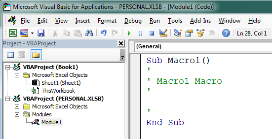
Press ALT+F11 to switch over to the Visual Basic Editor, then look at the top left hand corner of the editor window and see if you can spot the Project Explorer window. Press CTRL+R if you can't see it. Look for PERSONAL.XLSB in the listing and keep clicking the plus signs until you can see the modules in your Modules folder. Double-click on Module 1 to open it. If you have more than one of them (you've already been using your Personal Macro workbook) then double-click the one with the highest number. Select your recorded macro and Paste over it.

The Recorded macro viewed in the Visual Basic Editor

This is what your macro should look like. Notice how some of the words turn blue:

Macro pasted into the module

Save your Personal Macro workbook

Do this while you are in the Visual Basic Editor as it's tricky to do back in Excel. Click File, Save in the main menu. Press ALT+F11 to exit the editor and return to Excel.

Run the macro

Our macro is ready to go now so open the workbook file where you want to clean up all the text and then click View tab, Macros, View Macros. Choose PERSONAL.XLSB!Trimmer from the list and then click Run. Voila and Hey Presto! Quick as a flash your text is cleaned. Where did all those spaces go?

Your Personal Macro Workbook opens up automatically every time you start Excel so once you've saved it you can use it anytime you like. The Personal Macro workbook is a hidden workbook that's used to store handy macros that you would want to use on a regular basis, it's always open but it's not visible.

Commentary of the macro code

If you know all about macros then you can just copy the code and use it. If you want to analyse it then here's the explanation:

Firstly, we declare two object variables of class Range; rngText which is a collection of all the text cells in the active worksheet and rngItem, which is each individual text cell—each member of the collection.

Dim rngText As Range
Dim rngItem As Range

Then we initialise rngText using the Set keyword and loop through the collection with a For Each loop returning the cleaned text into each cell using the VBA Trim function.

Set rngText = Cells.SpecialCells(xlCellTypeConstants, 2)

For Each rngItem In rngText
rngItem.Value = Trim(rngItem.Value)
Next